
Power System Dynamics
Power System Dynamics
Power System Dynamics-Strip away all the formulas and one idea remains: a stable system, when nudged, comes back to rest; an unstable one runs away. The state-space model, the Jacobian, and the eigenvalues are simply the machinery that lets us answer that one question precisely. Let us build the idea from the ground up, adding mathematics only where it genuinely earns its place.
WHAT is stability?
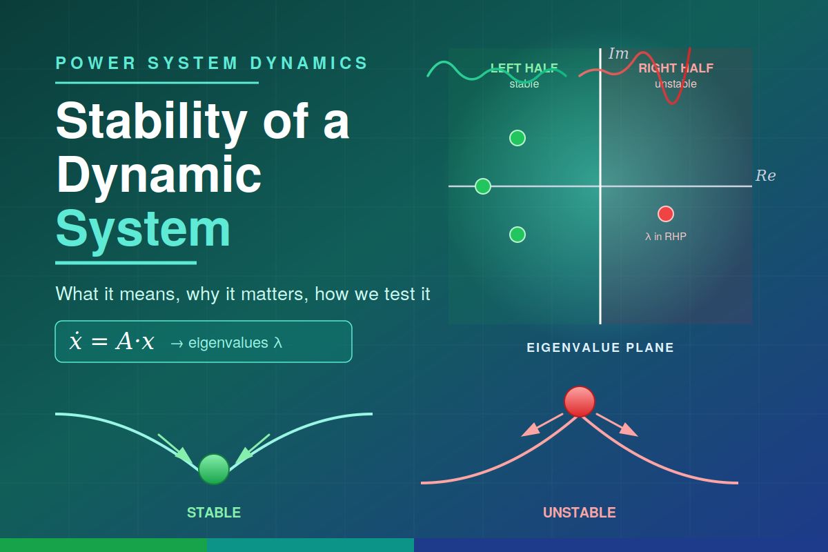
Imagine a ball in a valley and a ball balanced on a hilltop.
Push it a little and it rolls back to the bottom. The resting point is stable. Disturbances die out.
The slightest nudge sends it rolling away, never to return. The resting point is unstable. Disturbances grow.
A dynamic system is anything that changes over time according to a rule — a pendulum, a motor, a power grid. Its equilibrium is a resting state where nothing changes if left alone. Stability asks: if we disturb the system slightly from equilibrium, does it return (stable) or depart (unstable)?
Stable = disturbances shrink back to zero
Unstable = disturbances grow without bound
WHY does it matter?
Because instability means failure. An unstable aircraft tumbles, an unstable grid blacks out, an unstable reactor overheats, an unstable control loop oscillates until something breaks. Every engineered system that must stay doing its job depends on being stable.
This is why stability is not an afterthought but the very first thing an engineer checks. A beautifully accurate but unstable design is worthless.
HOW do we test for it?
Here the mathematics earns its keep. We follow four short steps: describe the system, find its equilibrium, linearize around it, and read off the eigenvalues.
Step 1 — Describe the system in state-space form
First we write down the rule of change. We collect every quantity that defines the system — positions, velocities, voltages, temperatures — into a single state vector x, and write how fast each one changes:
ẋ = f(x)
ẋ is the rate of change of the state; f is the rule (usually nonlinear) that the system obeys.
This compact form — one first-order equation in a vector — is the state-space representation. It works for a system with one variable or a thousand, which is why it is the standard language of dynamics.
Step 2 — Find the equilibrium
The equilibrium is the resting state where nothing changes — the bottom of the valley or the top of the hill. Mathematically, the rate of change is zero there:
f(xe) = 0
xe is the equilibrium point we want to test.
Step 3 — Linearize around the equilibrium
The rule f is usually a tangle of nonlinear terms, which is hard to analyse. But stability is only about small disturbances near xe — and near any point, a curve looks like a straight line. So we replace the curved rule with its straight-line approximation: a constant matrix A that captures the slope of f at the equilibrium.
The idea in one line: just as the slope of a curve y = f(x) at a point is its derivative, the “slope” of the vector rule f at xe is a matrix of derivatives called the Jacobian, written A.
Writing the small disturbance as Δx = x − xe, the dynamics near equilibrium become beautifully simple:
Δẋ = A·Δx
We have traded a hard nonlinear problem for an easy linear one — valid in the small neighbourhood where stability is decided. This is linearization, and it is the bridge from messy reality to clean analysis.
Step 4 — Read the eigenvalues
To see why a matrix tells us about stability, start with the simplest possible case: a single variable. Then A is just one number a, and the equation Δẋ = a·Δx has the famous exponential solution:
Δx(t) = Δx₀ · ea·t
Everything hinges on the sign of that one number:
ea·t shrinks toward zero. The disturbance fades and the system returns to rest.
ea·t grows without bound. The disturbance explodes and the system runs away.
A real system has many interacting variables, so A is a matrix rather than a single number. Hidden inside that matrix is a set of special numbers — its eigenvalues, written λ — and each one behaves exactly like the number a above. The matrix simply bundles several exponential modes together. Eigenvalues can be complex, λ = σ + jω, but only the real part σ plays the role of a, so only the real part decides stability:
All Re(λ) < 0 → every mode decays → STABLE
Any Re(λ) > 0 → one mode grows → UNSTABLE
Re(λ) = 0 → borderline — sustained oscillation, neither growing nor decaying
The imaginary part ω tells you whether the return is a smooth glide or a wobbling oscillation — but it never decides stability. Stability lives entirely in the real part.
The Whole Idea in One Picture
Plot the eigenvalues on a plane. A vertical line down the middle — the imaginary axis — divides the world in two:
If every eigenvalue sits in the left half, the system is stable. If even one strays into the right half, it is unstable. That single picture is the destination of all the mathematics — the state-space model, the equilibrium, the linearization, and the eigenvalues all exist to place dots on this plane.
In a nutshell
WHAT — Stability asks whether a disturbed system returns to rest or runs away.
WHY — Instability means failure: crashes, blackouts, explosions. It is the first thing to check.
HOW — In four steps:
1. Write the system as ẋ = f(x)
2. Find the equilibrium f(xe) = 0
3. Linearize to Δẋ = A·Δx
4. Check the eigenvalues of A — all real parts negative means stable; any positive means unstable.
Once the system is in linear state‑space form, stability can be determined using the A‑matrix.
Eigenvalue Analysis
The eigenvalues of matrix A determine stability:
Stability Conditions
- If all eigenvalues have negative real parts, the system is asymptotically stable.
- If any eigenvalue has a positive real part, the system is unstable.
- If eigenvalues lie on the imaginary axis, the system is marginally stable.
Interpretation
- Real part → damping
- Imaginary part → oscillation frequency
Example:
- Real part = –2 → stable
- Imaginary part = 5 → oscillation at 5 rad/s