
Numerical Integration Methods for Power System Stability
Numerical Integration Methods for Power System Stability Differential Equations
Power System Stability: When a large generator suddenly loses a transmission line or a fault clears after a few cycles, the rotor angles, speeds, and voltages of every machine in the grid begin to swing. The equations that govern these swings are nonlinear ordinary differential equations coupled with algebraic network equations. There is no closed-form solution — we cannot integrate them on paper. Instead, we step forward through time in small increments, computing the new state from the previous one. This stepping process is called numerical integration, and the choice of method decides whether the simulation finishes in seconds or hours, whether it converges or oscillates, and whether the answer is trustworthy.
The Equations We Must Solve
The classical machine model produces the swing equation for each generator:
where M is the inertia constant, δ is the rotor angle, Pm is mechanical input power, Pe is electrical output power, and D is damping. Because numerical methods work on first-order equations, we split this second-order equation into a pair:
dδ/dt = ω − ωs
dω/dt = (1/M) [ Pm − Pe(δ) − D(ω − ωs) ]
For an n-machine system, we get 2n such equations, plus additional equations for excitation systems, governors, and dynamic loads — easily several hundred state variables in a realistic study. The general form we are solving is:
0 = g(x, y)
The first row is the differential set (machine and controller dynamics). The second row is the algebraic set (network power-flow equations). This coupled structure is called a differential-algebraic equation system, or DAE, and it sits at the heart of every transient stability program.
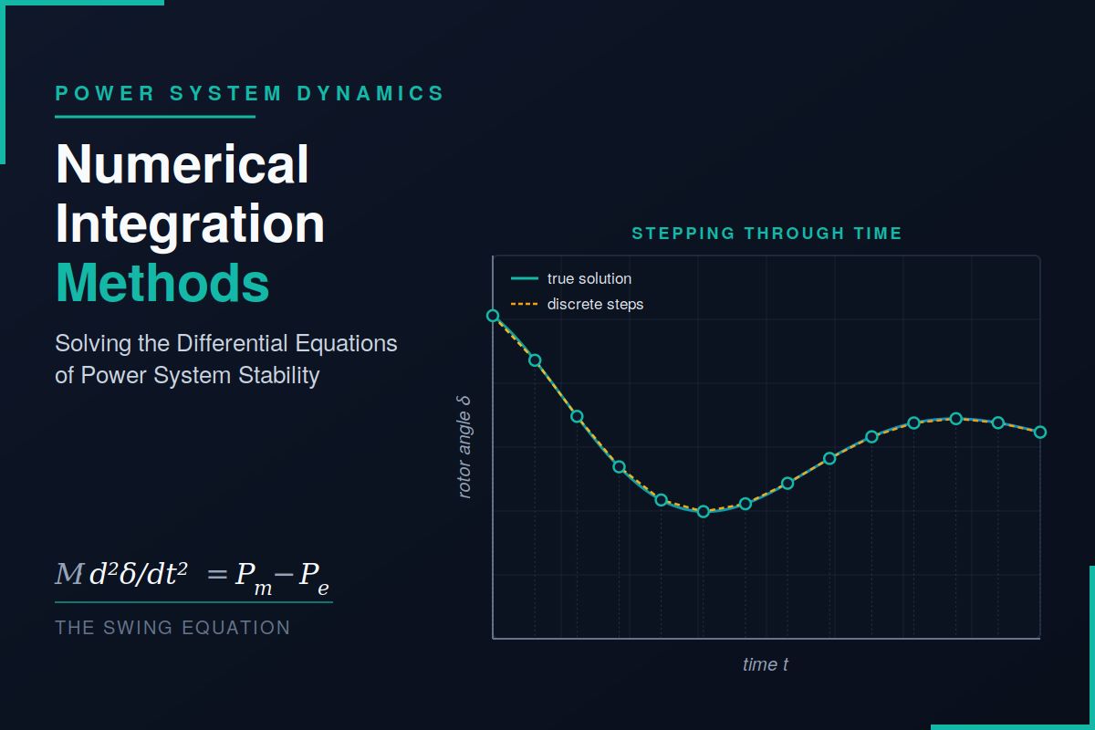
Numerical integration replaces the continuous derivative dx/dt with a discrete approximation. Given x at time t, we compute x at time t + Δt by estimating how much x changes over that small step. Every method differs only in how it estimates that change.
How Methods Are Classified
Before looking at individual methods, it helps to know the three classification axes engineers use:
| Distinction | Type A | Type B |
|---|---|---|
| Equation form | Explicit — xn+1 computed directly from known quantities at step n | Implicit — xn+1 appears on both sides; needs iteration to solve |
| Memory of past steps | Single-step — uses only the value at tn | Multi-step — uses values at tn, tn−1, tn−2, … |
| Step size | Fixed-step — Δt constant throughout the simulation | Variable-step — Δt adapts to local error or system stiffness |
Power-system programs sit at every corner of this cube. PSS/E classically uses an explicit single-step fixed-step method; EMTP-type programs use implicit trapezoidal integration; modern long-term dynamic simulators use implicit variable-step multi-step methods. Each choice trades accuracy, stability, and computational cost.
Euler’s Method — The Starting Point
The simplest possible idea: use the slope at the start of the interval and extend it as a straight line for the whole step.
Applied to the swing equation:
δn+1 = δn + Δt · (ωn − ωs)
ωn+1 = ωn + (Δt/M) · [ Pm − Pe(δn) − D(ωn − ωs) ]
Euler’s method is first-order accurate: the local truncation error per step is O(Δt²), and the cumulative error grows linearly with simulation length. This is too crude for serious stability work. With a step of 10 ms — typical for transient stability — Euler can drift several degrees in rotor angle over a one-second simulation, enough to flip a marginal case from stable to unstable.
Forward Euler is only numerically stable for very small Δt. For a system with eigenvalue λ, the requirement is |1 + λΔt| ≤ 1. With electromechanical oscillation frequencies near 1 Hz, that limits Δt to milliseconds — and the limit becomes brutal when fast subtransient or stator-flux dynamics are included.
Modified Euler — The Predictor-Corrector Idea
If a slope at the start of the interval is unreliable, average it with the slope at the end. The catch is that we don’t know the end value yet — so we estimate it first (predictor), then correct (corrector).
Step 1 — Predictor (forward Euler):
Step 2 — Corrector (average the two slopes):
This Heun’s method is second-order accurate (error O(Δt³) per step) at the price of two function evaluations per step. It is the workhorse for textbook transient stability examples because it is simple to code by hand yet noticeably better than plain Euler. Many old utility programs used modified Euler as their default integrator for decades.
Runge-Kutta Fourth-Order — The Industry Default
Heun’s method evaluates the slope twice. Runge-Kutta of order four (RK4) evaluates it four times, sampling at the start, two midpoints, and the end of the interval, then takes a weighted average.
k2 = f(xn + (Δt/2)k1, tn + Δt/2)
k3 = f(xn + (Δt/2)k2, tn + Δt/2)
k4 = f(xn + Δt·k3, tn + Δt)xn+1 = xn + (Δt/6) · (k1 + 2k2 + 2k3 + k4)
RK4 is fourth-order accurate — local error O(Δt⁵) — which means halving the step shrinks the error by a factor of sixteen. The four function evaluations cost more per step, but the larger usable step size makes RK4 cheaper overall than Euler for the same accuracy. RK4 with Δt = 10 ms gives angle accuracy of about 0.01 degree over a one-second simulation, more than sufficient for transient stability assessment.
RK4 is self-starting (no history needed), straightforward to code, and accurate enough that step-size control rarely matters for transient stability windows of 10-20 seconds. PSS/E, PowerWorld, ETAP, and DIgSILENT all offer RK4 (or a close cousin) as a standard option.
The Trapezoidal Rule — The Implicit Workhorse
All the methods so far are explicit. The trapezoidal rule averages the slopes at the start and end of the interval, just like Heun’s method, but it does not predict the end value first — it sets up the relationship directly:
Notice that xn+1 appears on both sides. This is an implicit equation. To solve it, we need Newton-Raphson iteration at each step, exactly the same machinery used in load flow. That sounds expensive — and per step, it is — but the payoff is enormous:
- The trapezoidal rule is A-stable. There is no step-size limit imposed by numerical stability; only accuracy decides Δt.
- It handles stiff systems — those with both very fast and very slow dynamics — without forcing tiny steps.
- It naturally accommodates the algebraic network equations because we are already iterating; the DAE is solved as one combined system.
The combined Newton-trapezoidal approach is the standard for electromagnetic transient programs (EMTP, PSCAD, ATP) and is increasingly used in long-term dynamic simulation where fast and slow dynamics coexist (governors, AGC, load tap changers, protection logic). The trapezoidal rule does have one well-known weakness — it is prone to numerical oscillations when applied to a step discontinuity, the so-called “trap-z hangover.” Modern programs use damping schemes or critical damping adjustment to suppress it.
Multi-Step Methods — Reusing the Past
Single-step methods like RK4 throw away all the slope information after each step. Multi-step methods keep the previous few slopes and fit a polynomial through them. The two main families are:
| Family | Character | Where Used |
|---|---|---|
| Adams-Bashforth (explicit) | Polynomial fit through past slopes, extrapolated to tn+1 | Predictor stage of P-C pairs |
| Adams-Moulton (implicit) | Polynomial includes slope at tn+1 | Corrector stage of P-C pairs |
| Gear / BDF (implicit) | Backward differentiation, stiffly stable | Stiff long-term simulators, voltage stability |
Gear’s backward differentiation formulas (BDF) are particularly important in voltage stability and long-term dynamic studies, where simulations may run for minutes of system time with both 100-ms electromechanical dynamics and 30-second tap-changer movements. BDF up to order six is implemented in commercial simulators like DSATools and Eurostag, usually with adaptive step and order control.
The Stiffness Problem
A system is stiff when it contains time constants spanning several orders of magnitude. Power systems are notoriously stiff:
| Phenomenon | Typical Time Scale |
|---|---|
| Stator electrical transients | 0.1 – 10 ms |
| Subtransient (damper winding) | 10 – 50 ms |
| Transient (field winding) | 0.5 – 10 s |
| Electromechanical swing | 0.1 – 2 s |
| Excitation and governor response | 0.05 – 5 s |
| Boiler thermal, load recovery | tens of seconds to minutes |
| Tap changers, AGC | minutes |
Explicit methods must use a step small enough for the fastest dynamic even when it has long since decayed. Implicit A-stable methods do not — they can take large steps once fast transients die down. This is why transient stability (focused on the 0.5–10-second window) often uses explicit RK4, while extended-term and voltage stability simulations use implicit methods.
Solving the DAE: Partitioned vs Simultaneous
The differential and algebraic equations can be solved in two architectures:
Partitioned (Alternating) Solution
At each step: solve algebraic equations first (network) with x held fixed, then advance x one step with y held fixed. Simple, modular, fits explicit methods naturally. Used in PSS/E classical mode. Risk: interface-error build-up if Δt is too large.
Simultaneous Solution
Differential and algebraic equations are combined into one large nonlinear system and solved together by Newton iteration. Inherently implicit. No interface error; larger step possible. Used in Eurostag and most EMTP-type tools.
Step Size — The Practical Heart of the Matter
Theory says smaller is better; practice says smaller is slower. The conventional step sizes that experienced engineers use as starting points are:
| Study Type | Method | Typical Δt |
|---|---|---|
| Classical transient stability | RK4 / modified Euler | 5 – 10 ms |
| Detailed model with subtransients | RK4 or implicit trap | 1 – 5 ms |
| EMT simulation | Trapezoidal (implicit) | 10 – 50 μs |
| Long-term/voltage stability | BDF, variable order | 0.1 – 10 s, adaptive |
A simulation that produces a clean, monotonic, well-damped curve is not automatically correct. Numerical damping — extra damping introduced by the integration scheme itself — can quietly hide a real instability. Always validate by halving the step and comparing; if the curves diverge, the larger step was wrong. This check costs one extra run but it has saved many engineers from approving an unstable design.
Comparison at a Glance
| Method | Order | Type | Stability | Best For |
|---|---|---|---|---|
| Forward Euler | 1 | Explicit | Conditional, tight | Teaching only |
| Modified Euler | 2 | Explicit P-C | Conditional | Simple TS studies |
| RK4 | 4 | Explicit | Conditional, generous | Transient stability default |
| Trapezoidal | 2 | Implicit | A-stable | EMT, stiff systems |
| Adams-Moulton (4) | 4 | Implicit multi-step | Good | High-accuracy non-stiff |
| Gear (BDF-2 to BDF-5) | 2 – 5 | Implicit multi-step | Stiffly stable | Long-term voltage stability |
A Worked Mental Example
Consider a single machine connected to an infinite bus through a transmission line. Let H = 5 s, ωs = 314.16 rad/s, Pm = 0.8 p.u., D = 0, and let a three-phase fault at the sending end reduce Pe to 0 during the fault and restore the pre-fault P-δ curve afterward. Pre-fault δ0 = 28.44°.
During the fault, the rotor accelerates uniformly because Pe = 0. With Δt = 10 ms and forward Euler:
dω/dt = (πf0/H) · (Pm − Pe) = (π·50/5) · 0.8 = 25.13 rad/s²
Δω = 25.13 × 0.01 = 0.2513 rad/s
Δδ = (ω − ωs) × Δt = 0 × 0.01 = 0 rad
δ1 = 28.44°, ω1 = 314.41 rad/s
After ten such steps (t = 100 ms, fault cleared) the Euler result is δ ≈ 31.7°. The RK4 result for the same Δt is δ ≈ 31.9° — closer to the analytic value of 31.94°. The 0.2° gap looks tiny on a single step but accumulates over the post-fault swing and can shift the critical clearing time by 5-10 ms. For a marginal stability case, that is the difference between a green and a red light.
Choosing a Method in Practice
A reasonable decision tree for the planning engineer:
- Short window (≤ 10 s), classical or two-axis models, no extremely fast dynamics → RK4 with Δt = 5–10 ms.
- Detailed subtransient models, HVDC, FACTS, power electronics → implicit trapezoidal with Newton iteration.
- Switching transients, lightning, breaker reignition → EMT trapezoidal at microsecond step.
- Long-term voltage stability, frequency response, AGC studies → variable-step BDF with order control.
- Real-time hardware-in-the-loop → fixed-step explicit (RK2 or RK4) for deterministic timing.
Closing Thoughts
Numerical integration is the invisible engine of every stability study. The same network and machine models, fed through different integrators with different step sizes, can produce subtly different conclusions — sometimes dangerously different. The competent stability engineer understands not just the equations, but the algorithm that solves them: its order of accuracy, its stability region, its sensitivity to step size, and the symptoms of trouble it can quietly mask.
Old hands have a saying: “Trust the simulator, but verify the integrator.” Run the same case twice with different step sizes, occasionally with a different method, and look at the trajectories side by side. If they agree, you have a result you can defend. If they disagree, the simulation is telling you something the equations alone never would.