Modelling of Excitation System Components

Modelling of Excitation System, Per Unit System, Field Testing for Model Validation and Verification

Modelling of Excitation System Components

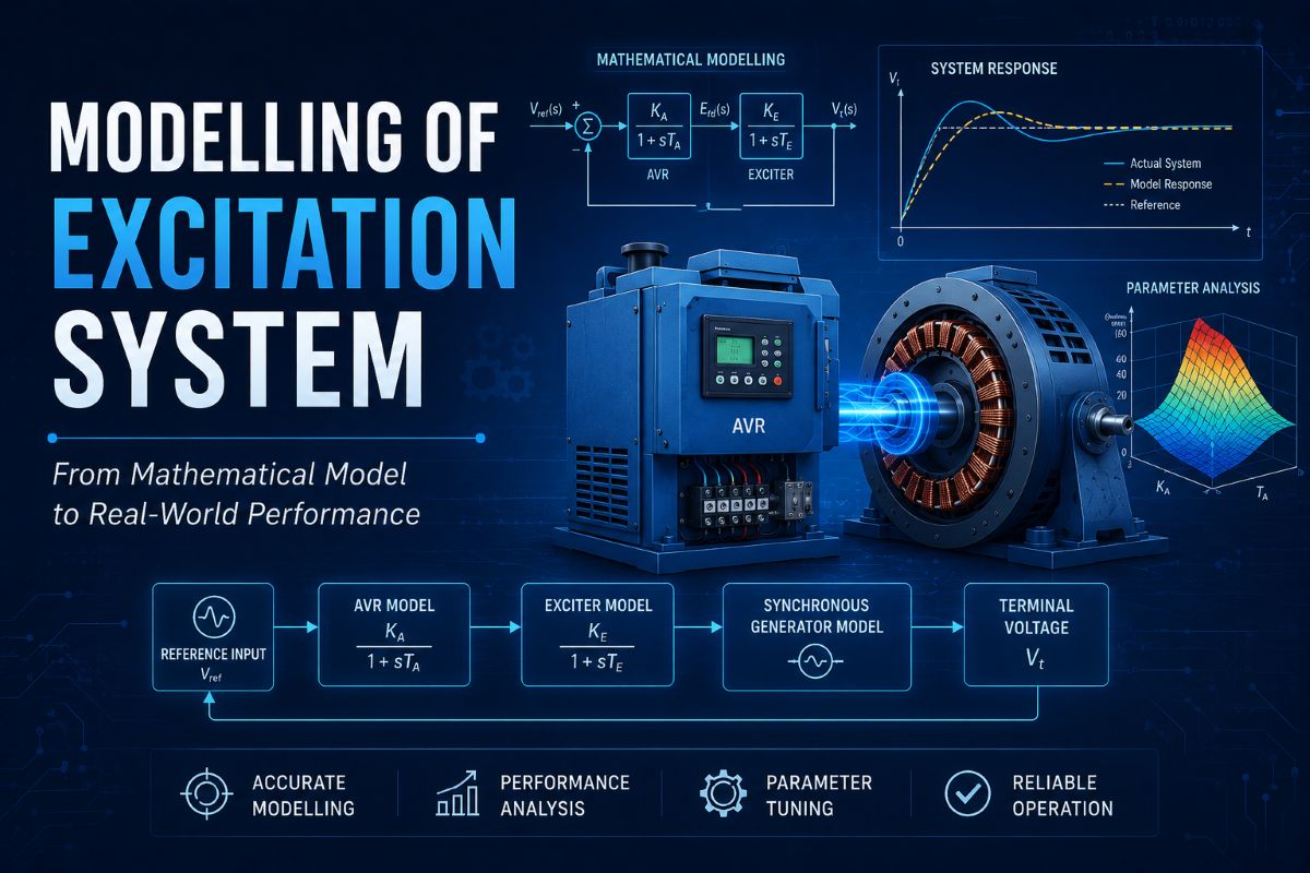
An excitation system model typically comprises several interconnected functional blocks, each representing a physical component or control function. The primary components modelled include the voltage regulator (AVR), the exciter (rotating or static), the power system stabiliser (PSS), and various limiters and protective functions. IEEE Std 421.5 provides standardised block diagram models that are widely adopted in power system simulation software.

Voltage Regulator Model: The automatic voltage regulator is modelled as a transfer function block that processes the error signal — the difference between the reference voltage and the measured terminal voltage. The model includes gain (K_A), time constants (T_A), and output limits (V_RMAX, V_RMIN). For digital AVRs, the model may incorporate lead-lag compensation blocks and proportional-integral (PI) control structures. The regulator model captures the dynamic response of the voltage control loop, including ceiling voltage capability and rate-limiting effects.

Exciter Model: The exciter converts the regulator output into field voltage applied to the synchronous generator. For DC exciters, the model includes the exciter’s self-excitation dynamics, saturation function S_E(E_FD), and the exciter time constant T_E. For static exciters that use controlled rectifiers fed from the generator terminals or an auxiliary source, the model is simpler — essentially a gain and time constant with source voltage dependency. Brushless AC exciter models incorporate the rotating rectifier dynamics and the alternator exciter’s voltage build-up characteristics.

Supplementary Control and Limiters: The PSS model is represented as a series of washout filters, lead-lag compensation stages, and a gain block. Its input may be rotor speed deviation, electrical power, or frequency. Limiters — including the overexcitation limiter (OEL), underexcitation limiter (UEL), and volts-per-hertz (V/Hz) limiter — are modelled as separate blocks that impose boundaries on the excitation system output to protect the generator from thermal or stability-related damage.

The Per Unit System in Excitation Modelling

Excitation system models are expressed in a per unit (pu) system to enable standardisation across generators of different ratings and to simplify mathematical analysis. In this system, all voltages, currents, and impedances are expressed as fractions or multiples of chosen base quantities.

The base quantities commonly used in excitation system modelling are defined on the generator’s stator side. The base stator voltage is the rated line-to-neutral RMS voltage, and the base stator current is the rated RMS stator current. The base field current (I_{FD base}) is defined as the field current required to produce rated terminal voltage on the air-gap line at no load. Similarly, the base field voltage (E_{FD base}) is the field voltage required to produce the base field current under steady-state conditions, accounting for field winding resistance.

Using this per-unit framework, the exciter output voltage E_FD at 1.0 pu corresponds to the field voltage needed to produce the rated terminal voltage at no load on the air-gap line. Under loaded conditions at rated power factor, the exciter output might be in the range of 2.5 to 3.5 pu, reflecting the additional field current required to overcome armature reaction and maintain rated voltage. Ceiling voltage is typically expressed as a per unit multiple, such as 3.0 to 5.0 pu, depending on exciter type and design requirements.

The per-unit system ensures that model parameters such as gains and time constants are directly comparable across different machines. When simulation software receives a per unit model, it can apply the model universally regardless of the specific machine ratings, provided the base conversions are correctly defined.

Field Testing for Model Validation and Verification

A model is only as useful as its ability to replicate the actual behaviour of the physical system. Field testing provides the measured response data against which the model is validated. IEEE Std 421.2 outlines recommended practices for the identification and testing of excitation system models.

Step Response Tests: The most common field test involves injecting a small step change (typically 1–5%) into the voltage reference input and recording the terminal voltage response over time. The measured response — including rise time, overshoot, settling time, and steady-state accuracy — is compared against the simulated response produced by the model. If the model is accurate, the simulated and measured waveforms should match closely.

Frequency Response Tests: By applying sinusoidal perturbations at various frequencies to the voltage reference and measuring the gain and phase of the terminal voltage response, a Bode plot of the open-loop or closed-loop transfer function can be constructed. This frequency domain characterisation reveals bandwidth, phase margin, and gain margin — essential indicators of stability and dynamic performance that can be directly compared with the model’s predicted frequency response.

On-Line Disturbance Recording: During actual system disturbances — such as line faults, load rejections, or switching events — digital fault recorders and continuous monitoring systems capture the real-time response of the excitation system. These recorded events serve as powerful validation scenarios because they exercise the model under realistic, complex conditions that a controlled test cannot easily replicate.

Model Verification Process: Verification involves iteratively adjusting model parameters until the simulated output matches the field test data within acceptable tolerances. Parameter identification techniques — including curve fitting, least-squares optimisation, and system identification algorithms — are applied to tune gains, time constants, and saturation characteristics. Once tuned, the model is cross-verified against a different set of test data to confirm that it generalises well and has not been over-fitted to a single test scenario.

Key Takeaway

The complete workflow of excitation system modelling — from constructing block diagram representations of the AVR, exciter, PSS, and limiters, through expressing all quantities in a standardised per unit framework, to validating the model against field-measured step responses, frequency response data, and disturbance recordings — ensures that simulation studies produce results that engineers and system operators can trust for real-world decision making.