
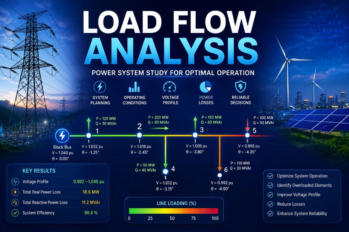
Load Flow Analysis
Load Flow Analysis Methods
Conceptual Understanding of Load Flow Analysis and Solution Techniques
📊 Introduction to Load Flow Analysis
Load flow analysis, also known as power flow analysis, is one of the most fundamental studies in power system engineering. It determines the steady-state operating conditions of a power system by calculating voltage magnitudes, voltage angles, and power flows through transmission lines and transformers under normal operating conditions.
The primary purpose of load flow studies is to ensure that the power system operates within acceptable voltage limits, with adequate reactive power support, without overloading transmission elements, and with sufficient margins for contingencies. This forms the foundation for system planning, operation, and control decisions.
⚡ Power Flow Network Equations: Conceptual Foundation
The power flow network equations represent the relationship between power injections at buses and the resulting voltage conditions throughout the system. At each bus in the network, two fundamental balance requirements must be satisfied:
Real Power Balance
The total real power injected at a bus (from generators) must equal the real power withdrawn (by loads) plus the real power flowing out through transmission lines. Any mismatch indicates a deficit or surplus that must be resolved by adjusting generation or changing network conditions.
Reactive Power Balance
Similarly, the reactive power injected must equal reactive power consumed plus reactive power losses. Reactive power management is critical for voltage support and stability. Insufficient reactive power leads to voltage collapse, while excessive reactive power causes voltage rise and equipment overstressing.
These balance equations must be satisfied simultaneously across all buses. The network equations form a set of nonlinear algebraic equations because power flow depends on both voltage magnitudes and angles in a nonlinear manner. This nonlinearity is why iterative solution methods are necessary.
🔗 Network Reduction: Simplifying Complex Systems
Concept: Network reduction is a preprocessing technique that simplifies the power system model by eliminating buses and branches that are not essential for the analysis being performed.
Why Network Reduction?
- Computational Efficiency: Fewer buses mean fewer equations to solve, dramatically reducing computation time
- Focus on Key Areas: Eliminates passive buses not relevant to study objectives, allowing concentration on critical regions
- Model Simplification: Reduces numerical issues and improves convergence characteristics
Types of Buses Eliminated:
Load Buses with No Injection: Buses that neither inject nor draw power can be removed without affecting the solution
Buses in Series: Two buses connected by a single transmission line with no intermediate generation or load can be combined into one
Radial Branches: Dead-end branches (radial lines) serving only loads or generation can be eliminated from the core network
Passive Intermediate Buses: Buses serving only as connection points with no power injection or withdrawal
Network reduction maintains the electrical characteristics of the remaining system while preserving solution accuracy for the elements of interest. After solving the reduced network, the eliminated buses can be restored through back-substitution to obtain complete system data.
🔄 Fundamental Theory of Solution Methods
Since power flow equations are nonlinear, they cannot be solved directly using simple algebra. Instead, iterative methods start with an initial guess and progressively refine the solution until convergence is achieved. All methods follow this fundamental principle: iterate until the power balance equations are satisfied within an acceptable tolerance.
Gauss-Seidel Method
Concept: An iterative approach where voltages at each bus are updated one bus at a time, using the most recently calculated values from previous buses in the same iteration. Think of it as a sequential update process where new information is immediately incorporated.
Advantages: Simple to understand and program, requires minimal memory, works well for radial networks
Disadvantages: Slower convergence, especially for large systems or heavily meshed networks; convergence becomes problematic when impedances are low
Best For: Small to medium systems, preliminary studies, problems with acceptable convergence characteristics
Newton-Raphson Method
Concept: Uses the principle of successive approximation with sensitivity information. It calculates how sensitive the power mismatch is to changes in voltage magnitudes and angles, then adjusts voltages proportionally to reduce mismatches. This is fundamentally more intelligent than simple sequential updates.
Advantages: Much faster convergence (quadratic convergence rate), handles both large and small systems efficiently, more robust for heavily meshed networks, and converges reliably even with difficult system configurations
Disadvantages: Requires computing sensitivity relationships, more complex programming, and greater memory requirements
Best For: Large interconnected systems, real-time operation, situations requiring fast solutions
⚙️ Decoupled Load Flow Methods
Fundamental Concept: The decoupling principle observes that in typical power systems, real power flows are primarily affected by voltage angles, while reactive power flows are primarily affected by voltage magnitudes. These two phenomena can be treated separately in a simplified manner, rather than solving the complete coupled system simultaneously.
Fast-Decoupled Load Flow (FDLF)
Approach: This method separates the problem into two independent sub-problems: one for voltage angles and real power, and another for voltage magnitudes and reactive power. Each sub-problem is solved iteratively.
Advantage over Newton-Raphson: By decoupling, the computational burden is distributed across simpler calculations, resulting in faster execution and reduced memory requirements while maintaining reasonable accuracy.
Key Benefit: Achieves a good balance between speed and accuracy. Computational time is typically 5-10 times faster than full Newton-Raphson while maintaining acceptable solution quality for operational studies.
Practical Application: Widely used in real-time energy management systems where fast solutions are critical for monitoring and control decisions within seconds.
📈 Method Selection Criteria
Use Gauss-Seidel: For small rural networks, preliminary screening studies, or when simplicity is valued over speed
Use Newton-Raphson: For large interconnected systems, comprehensive planning studies, contingency analysis, or when robustness is essential
Use Decoupled Methods: For real-time applications, online monitoring, quick studies where speed is prioritized, or large systems where computational efficiency is critical
Conclusion
Load flow analysis is the backbone of power system planning and operation. Understanding the conceptual foundations of power flow equations, network reduction techniques, and iterative solution methods enables engineers to select the most appropriate tool for their specific application. Modern power systems employ a combination of these methods depending on the time constraints, system complexity, and accuracy requirements of each study.