Power System Small Signal Stability
What is Small Signal Stability?
Every power system runs in a continuous state of balance. Generators produce exactly as much power as loads consume, voltages are held within acceptable bounds, and machine rotors spin in synchronism at the same effective electrical frequency across the entire interconnected network. This state of balance — where nothing changes — is called the operating point or equilibrium. In practice, the system is never perfectly undisturbed: loads switch on and off, generator outputs fluctuate slightly, and small transients propagate continuously through the network.
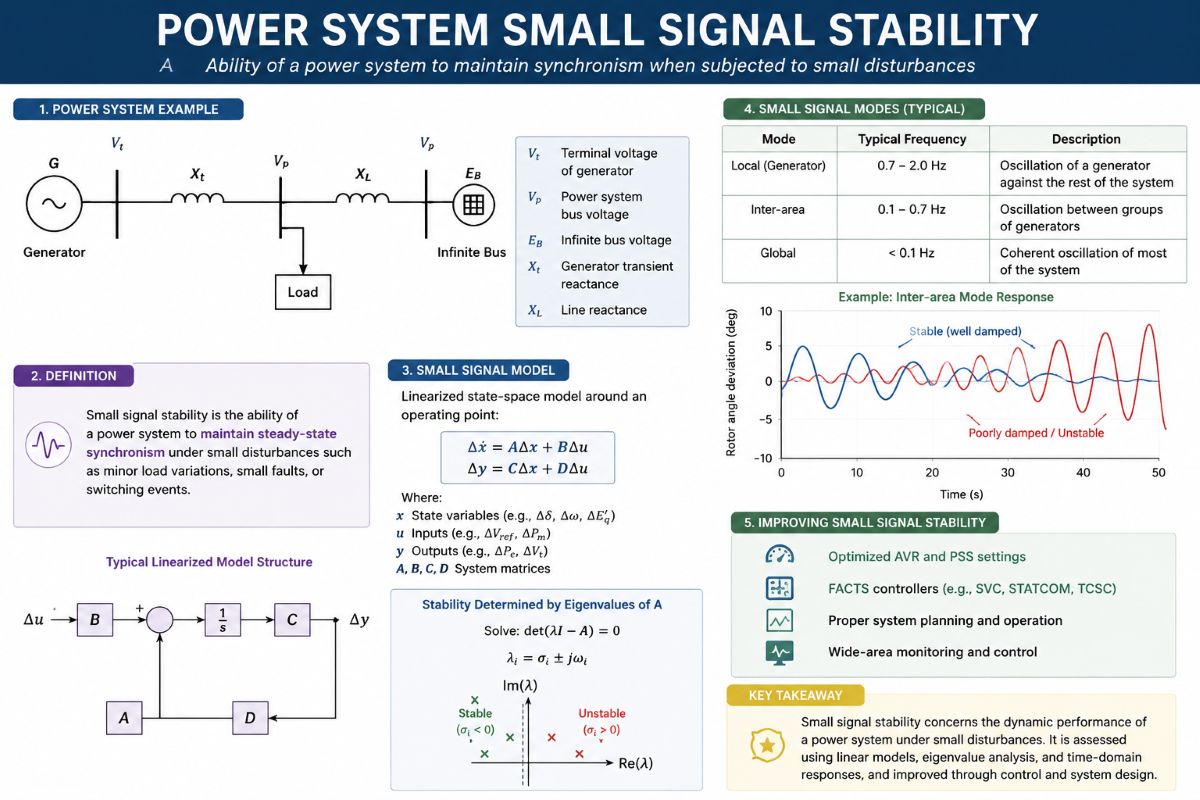
Small signal stability is the ability of a power system to return to its equilibrium condition after it experiences a small disturbance. The keyword is small — meaning a minor perturbation that does not dramatically alter the operating condition, such as a slight load change, a small reference adjustment on a voltage regulator, or a minor fluctuation in renewable generation output. The question is: after such a small nudge, does the system naturally settle back to its previous state, or do oscillations begin and grow over time?
This is deliberately distinguished from transient stability, which deals with large, sudden disturbances — a major fault, the loss of a large generator, or sudden disconnection of a transmission line. Transient stability is assessed through detailed time-domain simulation of the full nonlinear system behaviour. Small signal stability, by contrast, takes advantage of the fact that for genuinely small perturbations, the system can be treated as approximately linear near its operating point, which unlocks far more powerful and insightful analytical tools.
In large interconnected grids, groups of generators in different geographical areas can begin to swing against each other in a rhythmic back-and-forth — a phenomenon known as inter-area oscillation. These oscillations are typically slow, occurring between one and ten cycles per second. If they are well-damped, they fade away naturally. If they are poorly damped, they can persist or even amplify, ultimately threatening the synchronous cohesion of the entire grid. Small signal stability analysis is the engineering discipline that detects these conditions before they become a problem.
Steady-State Representation of a Dynamic System
To analyse a power system’s dynamic behaviour rigorously, engineers represent it as a dynamic system — a collection of quantities that evolve according to physical laws. These evolving quantities are called state variables. In a power system, state variables include things like the angular position of a generator rotor relative to a reference frame, the rotational speed of the rotor, the magnetic flux in the field winding of the machine, and the internal states of control systems such as the automatic voltage regulator and the governor.
The behaviour of these state variables is governed by the underlying physics — Newton’s laws for rotating masses, Faraday’s law for electromagnetic quantities, and the algebraic relationships of the electrical network. Taken together, these governing relationships form a complete description of how the system evolves from any given condition. The system also has inputs — quantities that are externally applied or controlled, such as mechanical power from a turbine or a voltage reference signal — and outputs — quantities of interest such as terminal voltage or electrical power delivered to the network.
The steady-state operating point is the specific set of values that all these state variables take when the system is in perfect balance — no machine is accelerating or decelerating, no voltage is rising or falling. This condition is established through a power flow calculation, which determines bus voltages, power flows, and reactive power conditions across the entire network for a defined generation and load scenario. The power flow solution then feeds into the machine equations to compute the corresponding rotor angles, field currents, and control system states for every generator. Together, these values constitute the complete steady-state description of the system at that operating point.
The steady-state operating point is not just a starting condition for simulation — it is the reference around which all small signal analysis is performed. Every conclusion drawn about stability, oscillatory behaviour, and control effectiveness applies specifically to this operating point. A different loading level, a different generation dispatch, or a different network configuration produces a different operating point and may yield entirely different stability characteristics.
Linearisation — Simplifying the System Near Its Balance Point
In a dynamic system (like a generator or power network), the state equation describes how internal variables change with time.
It looks like this:
Where:
- x = state variables (like rotor angle, speed, voltage, etc.)
- u = inputs (like mechanical torque, excitation voltage)
- f(x,u) = nonlinear function describing system behavior
This equation is nonlinear, meaning it involves products, sines, cosines, etc.
🔍 Linearization (Simplifying Around Operating Point)
To study small disturbances, we assume the system is near a steady operating point (x0,u0). We then expand f(x,u) using a Taylor series and keep only the first‑order (linear) terms:
Here:
- Δx=x−x0 → small change in state
- Δu=u−u0 → small change in input
- A and B are Jacobian matrices (partial derivatives of f)
This gives a linearised state equation valid for small signals.
🧠 Why It Matters
- The A‑matrix tells whether the system is stable (all eigenvalues have negative real parts).
- The eigenvalues of A correspond to modes of oscillation — frequency and damping.
- Engineers use these matrices to design controllers and stabilisers (like PSS).
The governing relationships of a power system are inherently nonlinear. The relationship between rotor angle and synchronising torque, the saturation characteristics of magnetic cores, the nonlinear voltage-current relationships of power electronics — none of these follow simple straight-line proportionality. Analysing nonlinear systems in full generality is mathematically demanding and often yields results that are difficult to interpret physically.
Linearisation exploits a fundamental insight: near any smooth operating point, a nonlinear relationship behaves approximately like a straight line. If you zoom in closely enough on a curve — any curve — it looks flat. This is the mathematical basis of linearisation. By restricting attention to small deviations from the operating point, the actual nonlinear governing relationships can be replaced by much simpler linear approximations that are accurate within that small neighbourhood. The resulting model describes not the absolute values of the state variables, but the deviations of those variables from their steady-state values.
The linearised model captures how each state variable’s rate of change depends on small deviations in all the other state variables and inputs. The strength of these interdependencies — how much a small change in one variable drives changes in another — is captured in a structured array of sensitivity coefficients. This array, known as the state matrix, is the mathematical heart of small signal analysis. It encodes, in compact form, the complete dynamic behaviour of the system for small perturbations around the operating point.
The state matrix is a compact representation of how all the state variables of the linearised system are coupled to one another. Its entries quantify the sensitivity of each variable’s rate of change to small perturbations in every other variable at the operating point. It is constructed from the partial derivatives of all governing relationships evaluated at the steady-state condition.
The input matrix describes how externally applied signals — such as a change in mechanical torque from the governor or a reference step on the excitation system — drive deviations in the state variables. It tells the analyst which inputs have the strongest leverage over which internal dynamics.
The output matrix maps internal state variable deviations to the measurable outputs of interest — terminal voltage deviation, frequency deviation, and power output change. It is needed when designing feedback controllers that act on observable quantities rather than internal states directly.
Analysing Stability — System Modes and Damping
Once the linearised model has been constructed around the operating point, the central question of stability can be answered analytically. The linearised system possesses a set of natural modes of response — characteristic patterns of behaviour that emerge spontaneously when the system is disturbed. These modes are the fundamental building blocks of the system’s dynamic response: any small disturbance will excite some combination of these modes, and the overall system response is the superposition of all excited modes evolving simultaneously.
Each mode has two defining characteristics: a frequency and a damping rate. The frequency tells how fast the mode oscillates — how many complete cycles it goes through per second. The damping rate tells whether the oscillation is growing, decaying, or staying at constant amplitude over time. These two characteristics together fully describe the qualitative behaviour of each mode.
When the damping rate of a mode is negative — meaning the mode naturally loses energy over time — the oscillation it produces will decay to zero. The system, after being perturbed, undergoes a diminishing back-and-forth and eventually returns to its original equilibrium. This is the desired behaviour. The faster the decay, the more robustly stable the mode is said to be.
When the damping rate of a mode is positive — meaning the mode gains energy over time — the oscillation it produces will grow progressively in amplitude. Left unchecked, this will eventually take the system far from its operating point, violating the assumption that the perturbation is small and potentially resulting in loss of synchronism or voltage collapse.
When the damping rate is exactly zero, the mode neither grows nor decays — the system oscillates indefinitely at constant amplitude. This condition is theoretically the boundary between stability and instability and is considered unacceptable in practice because any small increase in loading or change in operating condition can push the mode into instability.
Some modes produce no oscillation at all — the system simply drifts back toward equilibrium (stable) or drifts away from it (unstable) without any cyclic component. These non-oscillatory modes are associated with first-order time constants in the system — the speed with which a particular state variable returns to its steady-state value following a perturbation.
The damping ratio is a dimensionless number derived from the rate of decay and the frequency of oscillation of each mode. It expresses how quickly the oscillation dies out relative to how fast it oscillates. A damping ratio of zero means no decay; a ratio of one means the mode is critically damped with no oscillation at all. For power system electromechanical modes, the widely accepted engineering criterion is that the damping ratio must be at least five per cent under any credible operating condition to be considered adequately stable. Modes with damping ratios below this threshold are flagged for remedial action.
Modal Analysis — Identifying Which Machines Drive Each Mode
Determining that a mode is poorly damped tells the engineer that a problem exists. Modal analysis goes further and identifies where in the system the problem originates — which generators are swinging, in what pattern, and which machines are the dominant contributors to the problematic mode. Without this information, designing an effective remedy would require guesswork.
Every mode of the linearised system has an associated mode shape — a pattern that describes the relative amplitude and phase with which each state variable participates in that mode. Imagine several generator rotors all oscillating simultaneously during an inter-area mode. The mode shape reveals which rotors are moving in-phase with each other, which are moving in anti-phase, and which are barely moving at all. This spatial pattern is what defines the physical character of the oscillation — for example, it may reveal that generators in the northern region are swinging against generators in the southern region.
Participation factors refine this picture further. While the mode shape gives the oscillatory pattern across all state variables, the participation factor for each state variable in each mode gives a single number representing how strongly that variable is involved in that mode — regardless of the units or scaling of the variable. Participation factors are dimensionless and directly comparable across variables and machines, making them the preferred tool for identifying which generators need to be equipped with additional damping controls.
A generator with a high participation factor in a poorly damped mode is the primary candidate for installation of a Power System Stabiliser (PSS) — a supplementary controller that introduces a damping signal into the excitation system to actively suppress the oscillation. The participation factor-based identification closes the diagnostic loop: mode analysis reveals the frequency and damping of the problem; the mode shape and participation factors point directly at the machine where intervention is most effective.
Types of Oscillatory Modes in Power Systems
Not all oscillatory modes in a power system are of the same kind. Engineers classify them by their physical origin and oscillation speed, as each type demands a different analytical focus and a different remedial strategy.
These are the most challenging oscillations in large interconnected grids. They involve large coherent groups of generators — sometimes entire regional subsystems — swinging against each other across long transmission corridors. Because many machines are involved and the oscillations are slow and geographically spread out, inter-area modes are difficult to damp and require coordinated control action across multiple generators and substations. The collapse of the western North American grid in 1996 was partly attributed to poorly damped inter-area oscillations of this type.
These oscillations involve a single generator or power plant swinging against the rest of the network to which it is connected. They are faster than inter-area modes and are typically more localised in their physical extent. Because only one or a few machines are predominantly involved, local plant modes can usually be addressed effectively by installing a well-tuned Power System Stabiliser on the dominant machine identified through participation factor analysis.
These modes arise not from the electromagnetic and mechanical interaction of synchronous machines, but from the dynamics of the control systems themselves — excitation systems, governors, and power system stabilisers. Poorly tuned controllers can introduce modes whose state variables are predominantly the internal states of the control blocks rather than the physical rotor angles. Identifying these modes through modal analysis prevents the situation where a controller meant to improve stability actually introduces new instability.
These involve mechanical oscillations within the shaft system of a generator-turbine unit — the multiple masses of the high-pressure turbine, intermediate turbine, low-pressure turbine, and generator rotor twisting against each other along the mechanical shaft. They are particularly relevant for series-compensated transmission lines and HVDC systems, where electrical resonance can interact destructively with mechanical torsional frequencies in a phenomenon known as sub-synchronous resonance.
The Analytical Pipeline — From Operating Point to Grid Security
Small signal stability analysis follows a clear logical sequence. It begins with establishing the steady-state operating condition through a power flow solution. The system is then represented as a collection of coupled dynamic variables governed by nonlinear physical laws. Around the operating point, this nonlinear system is simplified into a linear model that accurately captures small perturbation behaviour. The linear model’s natural modes are then extracted — each described by a frequency and a damping rate. Modes with insufficient damping are flagged, and modal analysis identifies which machines and which parts of the system are responsible.
A critical limitation must always be kept in mind: the linearised model — and all stability conclusions drawn from it — is valid only in the immediate vicinity of the operating point from which it was derived. The power system operates across a wide range of conditions throughout the day and season, and across a vast number of possible network configurations following equipment outages. A mode that is adequately damped under peak load conditions may be poorly damped under light load, or when a major transmission line is out of service. Modern stability practice, therefore, requires that small signal analysis be performed across a comprehensive set of representative operating scenarios to build confidence that the system is robustly stable under all credible conditions.
Small signal stability analysis is a mandatory step in grid planning and operations — it underpins interconnection studies for new generation, the commissioning and tuning of Power System Stabilisers, the design of HVDC controls, and the integration of converter-interfaced renewable generation. As power systems evolve with increasing shares of inverter-based resources, the interaction between fast power electronic control loops and traditional synchronous machine dynamics is introducing new types of oscillatory phenomena that are extending and challenging the classical small signal framework.