Fundamental Power Flow Analysis
Power Flow Analysis: The First Assumption and How the Method Proceeds
Before a single voltage is calculated, power flow analysis rests on one quiet but decisive assumption. Understanding what it is — and why it is unavoidable — is the key to understanding the entire method.
What is power flow analysis trying to find?
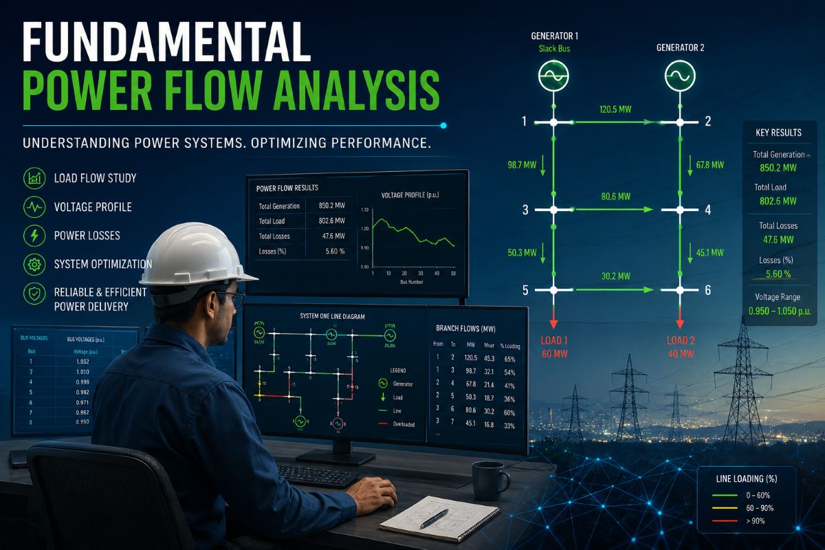
A power system is a network of generators, transmission lines, and loads, all interconnected at points called buses. Power flow (or load flow) analysis answers a deceptively simple question:
“Given the generation and load at every point in the network, what is the steady-state voltage at each bus, and how much power flows through every line?”
Once the voltage magnitude and angle are known at every bus, everything else falls out of them: line flows, transmission losses, generator loading, and whether any equipment is over- or under-stressed. The voltages are the answer; everything else is bookkeeping built on top of them.
Four quantities live at every bus
To see where the central assumption comes from, start with the bus itself. At any bus in the system, there are exactly four electrical quantities that describe its condition:
|V| — Voltage magnitude How strong the voltage is | δ — Voltage angle It’s phase relative to a reference |
↑ A BUS (node) in the network ↓ | |
P — Real power net active power injected | Q — Reactive power net reactive power injected |
Every bus is described by these four numbers: |V|, δ, P and Q.
The crucial rule: at every bus, exactly two of these four quantities are known (specified in advance) and the other two are unknown (to be calculated). Which two are known is decided by the physical nature of the bus.
One bus must be the “slack” bus
The very first assumption in power flow analysis — the one everything else depends on — is that one bus is chosen as the slack bus (also called the swing or reference bus), and its voltage is fixed in advance at a reference value, typically 1.0 per unit at an angle of 0°.
This is not a mathematical convenience. It is forced on us by the physics of the network. Here is why.
The chicken-and-egg problem of losses
In any power system, the books must balance. The total power generated has to equal the total power consumed by loads plus the power lost as heat in the transmission lines:
Total Generation = Total Load + Transmission Losses
The trap is hidden in that last term. The losses are the I²R heating in every line. They depend on the line currents, which depend on the power flows, which depend on the bus voltages — and the bus voltages are exactly what we are trying to calculate. So the losses cannot be known until after the problem is solved, yet balancing generation against load needs them before we start.
If we tried to specify the real power output of every generator in advance, we would be fixing the total generation before we know the losses. The equation above would then refuse to balance, and the problem would have no consistent solution.
The way out is elegant. We pick one generator bus and deliberately refuse to fix its power. Instead, we fix its voltage magnitude and angle. This bus then automatically supplies whatever extra power is needed — including the unknown losses — to make the books balance. It “takes up the slack,” which is exactly how it earns its name.
Bus 1 — SLACK |V| and δ fixed supplies the balance | Bus 2 — PV P and |V| fixed a generator bus |
↕ Transmission lines — the loss on every line is unknown until the system is solved ↕ | |
Bus 3 — PQ P and Q fixed a load bus | Bus 4 — PQ P and Q fixed a load bus |
Because every line loss is unknown until the solution is found, one bus (Bus 1) keeps its voltage fixed and absorbs the imbalance.
The slack bus plays a second, equally important role. AC voltages only have meaning relative to one another, so we need a common angle reference. By fixing the slack bus angle at 0°, every other bus angle in the system is measured against it. The slack bus is therefore both the power balancer and the angular anchor of the whole network.
Classifying the buses: who knows what
With the slack bus settled, the rest of the buses are sorted by what the physical equipment naturally holds constant. This gives three bus types, each with a different pair of known quantities.
| Bus type | |V| | δ | P | Q | Typical example |
|---|---|---|---|---|---|
| Slack / Swing | Known | Known | Unknown | Unknown | Reference power plant |
| PV (generator) | Known | Unknown | Known | Unknown | Generator with AVR holding voltage |
| PQ (load) | Unknown | Unknown | Known | Known | Substation feeding consumers |
Green cells are specified in advance; amber cells are what the analysis must calculate. The vast majority of buses in a real system are PQ load buses.
The logic behind each type is physical. A generator bus has an automatic voltage regulator holding its terminal voltage and a governor setting its real power, so P and |V| are the natural knowns — hence PV. A load bus draws a known active and reactive demand, but its voltage sags or rises depending on the network, so P and Q are known, and the voltage is the unknown — hence PQ.
How the analysis then proceeds
With the assumptions in place, the method follows a clear sequence. Each step builds on the previous one.
Steps 4 and 5 form the iterative loop — the heart of every power flow program.
Why must the solution be iterative?
The relationship between power and voltage in an AC network is fundamentally non-linear — power depends on the product of voltages and on the sine and cosine of angle differences. There is no clean, one-shot formula that simply hands back the bus voltages.
So the method starts from the flat-start guess, calculates how badly that guess violates the power balance at each bus (the mismatch), corrects the voltages to shrink that mismatch, and repeats. Each pass brings the estimate closer to the true answer. When the mismatch becomes negligibly small, the solution has converged and the bus voltages are accepted as final.
The thread that ties it together
Everything in power flow analysis traces back to one honest admission: we cannot know the transmission losses in advance. That single fact forces us to nominate a slack bus, fix its voltage, and let it balance the system. From there, classifying the remaining buses, guessing a flat start, and iterating to convergence is simply the disciplined way of solving for the voltages the slack bus assumption left open.
Get the Slack bus right, and the rest of the method is a logical staircase from one step to the next.