Power Flow Analysis Procedure
Power Flow Analysis Procedure
Power flow analysis, also called load flow analysis, answers a deceptively simple question: given the generation and the load at every point in a network, what voltage appears at each busbar and how much power flows through each line and transformer? It is the most fundamental study in power system engineering, the starting point from which planning, operation, and protection all proceed. Because the relationship between voltages and power flows is non-linear, the answer cannot be written down directly; it must be found by repeated, iterative calculation until the numbers settle.
The Power Flow Analysis Procedure
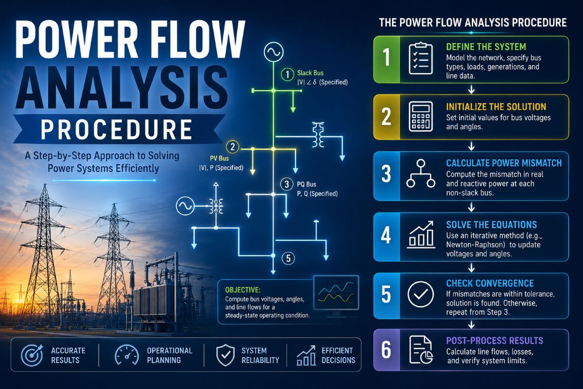
Every busbar in the study is first classified into one of three types. The slack or swing bus is the reference: its voltage magnitude and angle are fixed, and it makes up whatever generation is needed to balance the system’s losses, which are not known until the solution is complete. A voltage-controlled (PV) bus is where a generator holds a specified voltage while injecting a specified real power. A load (PQ) bus is where both the real and reactive power are known — typically a point of demand — and the voltage is the unknown to be found.
The job of the power flow is to find the two unknowns at every bus that were not specified — voltage angle and magnitude at load buses, and reactive power and angle at generator buses — so that power balances everywhere.
With the buses classified and the network’s interconnections assembled into an admittance description, the solution proceeds by iteration. An initial guess is made for the unknown voltages, the resulting power injections are computed and compared with the specified values, and the voltages are corrected to reduce the mismatch. This repeats until the mismatch falls below a small tolerance. Several methods carry out this loop: the Gauss-Seidel method is simple but slow; the Newton-Raphson method converges quickly and reliably and is the workhorse of large studies; and the fast-decoupled method exploits the weak coupling between real power and voltage magnitude to speed the calculation further. Once converged, the study reports every bus voltage, every line flow, the losses, and the slack-bus generation.
Pre-Fault Power Flow
The pre-fault power flow is the base case: the steady-state solution of the system as it normally operates, with all equipment in service and load and generation set to a chosen condition such as peak demand. It establishes the healthy operating point — the voltage at every bus and the loading of every line under intact conditions — and confirms that voltages sit within limits and no element is overloaded before any disturbance is considered.
This base case matters for two reasons. It verifies that the system is being operated within its design limits, and it provides the reference against which the effect of any disturbance is measured. In stability studies it also fixes the initial conditions of the machines — their rotor angles and power outputs at the instant just before a fault occurs.
Post-Fault Power Flow
A post-fault power flow is the steady-state solution of the system after a disturbance has occurred and the protection has acted to clear it — usually by tripping the faulted line, transformer, or generator. With that element removed, the same load must now be carried by the remaining network, and a fresh power flow is solved to find the new voltages and flows in this weakened configuration.
The post-fault case reveals whether the surviving network can carry the redistributed load safely. Lines that were comfortably loaded before the fault may now be overloaded, and voltages that were healthy may now sag below limits.
This is the basis of contingency analysis, in which the loss of each major element is simulated in turn, and a post-fault power flow is solved for each. The widely used N-1 criterion requires that the system remain within limits after the loss of any single element, so the post-fault flows of every credible contingency are checked against thermal and voltage limits. Where a post-fault case violates a limit, operators must adjust the pre-fault dispatch — rescheduling generation or arming corrective actions — so that the system would still be secure if that fault actually happened.
In short, the pre-fault power flow describes the system as it stands, and the post-fault power flow describes the system as it would be left after a disturbance. Comparing the two is how engineers judge whether a network is operating not merely correctly, but securely — able to withstand the loss of any single part without distress.