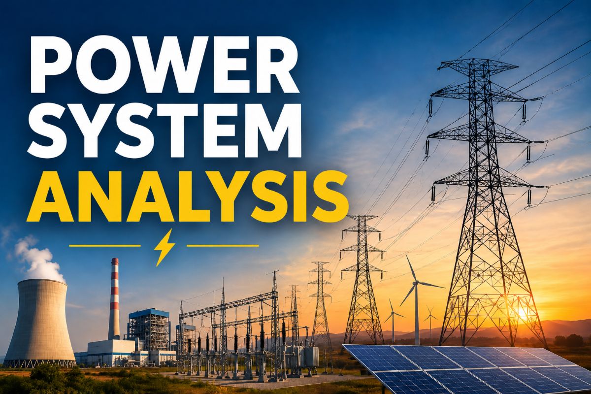
Power System Analysis
Power System Analysis: From Load Flow to Transient Stability — A Complete Beginner’s Guide
Power system analysis is the backbone of electrical grid planning, operation, and protection. It splits into two main branches: steady-state analysis (power flow) and dynamic analysis (transient stability). Understanding both — and how they connect — is essential for every electrical engineer.
What Is Power Flow Analysis?
Power flow analysis, also called load flow analysis, is a steady-state study that determines the operating point of an electrical grid. It calculates:
Voltage magnitude and angle at every bus
Real and reactive power flow in every transmission line
Total system losses
Whether the equipment is loaded within its thermal and voltage limits
Engineers use it daily to answer the question: “Can the grid deliver the required load today while keeping voltages in range and lines under their limits?”
The Ybus Matrix: The Circuit’s DNA
Before solving anything, the physical network must be converted into a mathematical model. This is done using the bus admittance matrix, commonly called Ybus.
What is Ybus?
Ybus is a square matrix where each row and column represents a bus in the network. It contains admittance values (Y = 1/Z) that describe how buses are connected.
Diagonal elements (Yii): Self-admittance of bus i. It is the sum of all admittances connected to that bus.
Off-diagonal elements (Yij): Mutual admittance between bus i and bus j. It is the negative of the admittance directly connecting them. If no direct connection exists, it is zero.
Why is it useful?
Ybus compactly represents the entire network. Once built, it allows us to write a simple equation:
Where I is the vector of current injections at each bus, and V is the vector of bus voltages. In power flow, we work with power rather than current, so we use the power equation
Types of Buses and How They Are Used in Analysis
In power flow studies, buses are classified based on which two quantities are known beforehand and which two the solver must find.
At every bus, there are four variables: P, Q, |V|, and δ. The power flow equations can only solve for two unknowns per bus, so we must specify two. The classification tells the solver what to fix and what to find.
How Power Flow Is Done: The Newton-Raphson Method
The power flow equations are non-linear. They cannot be solved directly with simple algebra. Engineers use iterative numerical methods, and the Newton-Raphson method is the most popular.
How it works (in simple terms):
Start with a guess for all unknown voltages and angles (usually 1.0 pu and 0°).
Calculate the mismatch between the scheduled power (P, Q) and the power calculated from the current voltage guess.
Use the Jacobian matrix (a matrix of partial derivatives) to determine how much to adjust the voltages and angles to reduce the mismatch.
Update the voltages and angles and repeat.
Stop when the mismatch is smaller than a very tiny tolerance.
Newton-Raphson is preferred because it converges rapidly (usually in 3–7 iterations) and is reliable for large systems.
Voltage Profile and Line Loading
Once the solver converges, engineers analyze two key outputs:
Voltage Profile
This is the voltage magnitude at every bus plotted in a chart or table. Utilities typically require voltages to stay within ±5% of nominal (0.95 to 1.05 pu). If a bus voltage is too low, it may indicate:
Heavy loading
Weak transmission paths
Insufficient reactive power support
Line Loading
This is the percentage of a transmission line’s thermal or stability rating that is being used. If loading exceeds 100%, the line overheats or becomes unstable. Power flow tells operators which lines are approaching their limits so they can reroute power or reinforce the network.
What Is Transient Stability?
Transient stability is the ability of a power system to remain in synchronism after a large, sudden disturbance. Examples include a three-phase short circuit, the sudden loss of a large generator, or the tripping of a major transmission line.
Unlike power flow, which is a static snapshot, transient stability is a dynamic study that examines the first few seconds after a fault. The central question is: “After the disturbance is cleared, will the generators swing back together, or will they pull apart and lose synchronism?”
The Power Angle Curve
The core physics behind stability is the power-angle relationship. For a single machine connected to an infinite bus:
- Pₑ = electrical power delivered to the grid
- E = generator internal voltage
- V = infinite bus voltage
- X = total reactance between them
- δ = power angle (the angle between E and V)
This is a sine curve. It reaches its maximum at δ = 90°, which is the steady-state stability limit. Normal operation is at δ₀ = 20° to 40°, leaving a comfortable margin.
If the angle increases beyond 90° during a disturbance, the electrical power output actually decreases while the mechanical input from the turbine stays roughly constant. The generator then accelerates uncontrollably and loses synchronism.
The Swing Equation
The motion of the generator rotor is governed by the swing equation:
Where:
M = inertia constant (reflects the rotor’s stored kinetic energy)
Pₘ = mechanical power input from the turbine
Pₑ = electrical power output (from the power-angle curve)
This is simply Newton’s second law applied to a rotating mass. If the turbine produces more power than the grid can absorb (Pₘ > Pₑ), the rotor accelerates and δ increases. If the grid absorbs more than the turbine produces (Pₘ < Pₑ), the rotor decelerates and δ decreases.
The Equal Area Criterion: A Simple Energy Test
Instead of solving the swing equation numerically for simple systems, engineers use the Equal Area Criterion (EAC). It is a graphical energy-balance method that works on the power-angle curve.
The Setup
During a typical fault sequence, we draw three curves on the P-δ diagram:
Pre-fault curve — the normal sine curve
During-fault curve — much lower because the voltage has collapsed
Post-fault curve — lower than pre-fault because the network topology has changed (e.g., a line is lost)
We also draw a horizontal line at Pₘ (mechanical power, which is roughly constant).
The Two Areas
A₁ (Accelerating Area): The area between the Pₘ line and the during-fault curve, from the initial angle δ₀ to the clearing angle δc. This represents the excess energy that speeds up the rotor during the fault.
A₂ (Decelerating Area): The area between the post-fault curve and the Pₘ line, from the clearing angle δc to the point where they cross again. This represents the energy the system can absorb to slow the rotor down.
The Stability Rule
If A₂ ≥ A₁, the system is stable. The rotor reaches a maximum angle and swings back.
If A₂ < A₁, the system is unstable. The rotor overshoots the available decelerating energy and keeps accelerating.
Critical Clearing Angle (δcc): The maximum angle at which the fault can be cleared such that A₂ exactly equals A₁. The corresponding time is the Critical Clearing Time (CCT) — the protection system must operate faster than this.
Connecting Power Flow and Transient Stability
These two studies are not separate silos. They are sequential steps in the same workflow:
Power flow provides the starting point. The initial angles δ₀ calculated in the load flow are the angles at which the rotors sit before the fault. Transient stability then tests what happens if a shock pushes them away from that starting point.
Practical Summary
Power flow analysis tells you if the grid works on a normal day. It uses the Ybus matrix, classifies buses as PQ, PV, or Slack, and solves with the Newton-Raphson method. The results — voltage profile and line loading — confirm whether the system is healthy.
Transient stability tells you if the grid survives a crisis. It uses the power-angle curve, the swing equation, and the equal area criterion to determine whether generators remain in sync after a fault. The key is whether the decelerating area can absorb the accelerating area before the rotor swings past the point of no return.
Together, they form the complete picture: power flow is the map, and transient stability is the crash test. Both are built on the same foundation — the power-angle relationship and the network admittance model.