Power Flow Analysis In AC DC Systems
Power Flow Analysis
In AC DC Systems
Power Flow Analysis In AC DC Systems-Formulation of the DC link model, the per-unit system for DC quantities, unified and sequential solution strategies, and a worked four-terminal DC system example.
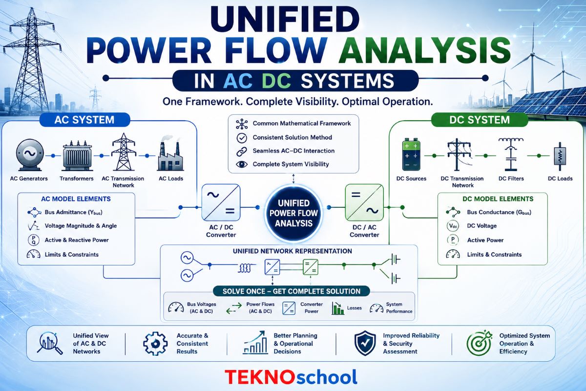
Power flow analysis — also called load flow analysis — is the computational determination of the steady-state voltages, currents, and active and reactive power flows throughout a network under specified generation and load conditions. For a purely alternating current network, the problem is well understood and solved by Newton-Raphson or fast-decoupled methods applied to the nodal admittance equations. When one or more HVDC links are embedded in that AC network, the problem is fundamentally enlarged: the converter stations introduce additional variables (DC current, DC voltage, firing angle) and additional equations (converter characteristics, control mode constraints) that must be solved simultaneously with, or iteratively alongside, the AC bus equations.
The coupling between the AC and DC subsystems is bidirectional. The DC link absorbs active power from the rectifier AC bus and delivers it to the inverter AC bus; at both terminals, it also consumes reactive power that depends on the operating angle and must be supplied by the local AC network or by switched compensation. Changes in the AC bus voltage alter the converter operating point, and changes in the converter firing angle alter the reactive power drawn from the AC bus. This mutual dependence means that neither the AC power flow nor the DC load flow can be solved independently in the general case.
At every converter terminal, the AC/DC interface is characterized by three exchanged quantities: the AC bus voltage magnitude (which determines the converter no-load DC voltage Vd0), the DC current Id (which determines the reactive power demand and the commutation voltage drop), and the converter reactive power Qc (which appears as a load on the AC bus power balance).
Two broad solution philosophies exist. In the sequential (alternating) method, the AC power flow and the DC load flow are solved in alternating outer iterations, with each solution feeding updated boundary values to the other. In the unified method, the DC converter equations are incorporated directly into the Newton-Raphson Jacobian of the AC system, and all variables are updated simultaneously in each iteration. The unified approach converges faster but requires more complex Jacobian coding; the sequential approach is simpler to implement and is adequate when the DC system is small relative to the AC network.
Converter and Line Equations for Steady State
Each converter in the DC link is described by its fundamental-frequency steady-state characteristic. For a twelve-pulse line-commutated converter (two six-pulse bridges in series), the DC terminal voltage is related to the AC commutating bus voltage Vk, the converter transformer off-nominal turns ratio ak, the commutation reactance Xck, the DC current Id, and the firing angle αk (rectifier) or extinction angle γk (inverter) by:
Vdk = (3√2 / π) ak Vk cos αk − (3/π) Xck Id
For the rectifier, replace α with γ for the inverter minimum extinction angle constraint
The active power drawn from AC bus k by the converter is Pk = Vdk Id (neglecting valve losses). The reactive power consumed is Qk = Pk tan φk, where the power factor angle φk is approximated from the overlap angle μk and the firing or extinction angle. In practice, Qk is bounded by the rating of the switched reactive compensation installed at the converter bus, and the compensation switching steps must be modelled as discrete variables in an outer loop.
The DC transmission line connecting the rectifier and inverter terminals is represented by its lumped resistance Rdc. For a two-terminal link, this gives a single constraint equation. For a multi-terminal network, the DC node voltages Vdi and the DC currents flowing in each branch Ib are related by a DC nodal conductance matrix Gdc analogous to the AC Y-bus, and the DC bus voltages are the solution of:
Gdc Vdc = Idc
where Idc is the vector of converter current injections at each DC node
Each converter also operates under a specified control mode. Common modes are: constant DC current (the rectifier holds Id at its ordered value by adjusting α), constant DC voltage (one inverter regulates Vd by adjusting γ), and constant power (the rectifier adjusts α to maintain Pdc at its set point). The control mode determines which variable is specified and which is the unknown in each converter’s equation set, and must be assigned before the DC load flow is formulated.
Iterative Solution with Fixed AC Bus Voltages
When the AC bus voltages are treated as known (either from a preceding AC power flow solution or as specified boundary conditions), the DC load flow becomes a set of nonlinear algebraic equations in the DC unknowns. The unknowns typically include the DC bus voltages Vdk, the common DC current Id (two-terminal) or the individual branch currents (multi-terminal), and the converter angles αk or γk.
For a two-terminal link, convergence typically requires fewer than five iterations because the equation set is small and nearly linear in the vicinity of the operating point. For multi-terminal systems, the cross-coupling between converters through the DC network makes convergence slower, and damping of the iteration updates (using a relaxation factor between 0.5 and 0.9 on the DC current update) is often needed to prevent oscillation.
Transformer tap ratios ak are treated as a discrete outer loop: once the continuous solution has converged, the tap is rounded to the nearest physical step, the solution is re-run, and the new reactive power injection Qk is re-evaluated. This outer tap adjustment loop is repeated until no tap changes are required.
Selecting DC Base Quantities
Expressing DC quantities in per-unit consistently eliminates the numerical disparity between high voltage (hundreds of kilovolts) and small current (kiloamperes) values, simplifies convergence checking, and allows the DC network equations to be combined with the AC network equations in a common numerical framework.
The standard choice is to select a DC base voltage Vdc, base equal to the rated DC voltage of the link, and a DC base power Sdc, base equal to the rated power of the link. The base DC current and base DC resistance then follow directly:
| Quantity | Base Definition | Relationship |
|---|---|---|
| DC Voltage | Vdc,base = rated DC pole-to-pole voltage | Chosen freely; typically 500 kV or 800 kV |
| DC Power | Sdc, base = rated link power | Usually set equal to Sac, the base of the AC system |
| DC Current | Idc, base = Sdc, base / Vdc, base | Derived; ensures Ppu = Vpu × Ipu |
| DC Resistance | Rdc,base = Vdc,base2 / Sdc,base | Consistent with Ohm’s law in pu: Vpu = Ipu Rpu |
The converter characteristic equation in per unit retains the same form as in physical units, with Vd0,pu = (3√2/π) apu Vk,pu, where Vk,pu is the AC bus voltage in the AC per-unit system and apu is the transformer turns ratio expressed as the ratio of actual turns ratio to the base turns ratio (Vdc, base / Vac, base × π/3√2). This scaling ensures that when both AC and DC voltages are at their respective rated values and the firing angle is zero, Vd0,pu = 1.0.
Using the same Sbase for both AC and DC subsystems simplifies the power mismatch equations at the converter terminal buses, since the active power extracted from the AC bus and the active power injected into the DC network are equal in per unit (minus losses), and no scaling factor appears in the interface equations.
Unified Newton-Raphson Formulation
In the unified method, the DC converter equations are appended to the AC power flow mismatch vector and the DC unknowns are added to the state vector updated in each Newton-Raphson iteration. If the AC system has nAC buses and the DC system has nDC converter terminals, the combined mismatch vector has the form:
[ ΔPAC | ΔQAC | ΔPdc | ΔQdc | Δfconv ]T = −J Δx
where Δfconv are the converter characteristic mismatches and J is the extended Jacobian
The extended Jacobian J has the standard AC sub-blocks in its upper-left partition, coupling terms between AC bus voltages and converter reactive power in the off-diagonal partitions, and converter equation partial derivatives in the lower-right partition. The coupling terms are generally sparse: only the converter terminal buses have nonzero entries in the AC-to-DC coupling sub-blocks, so the overall sparsity of the Jacobian is only marginally reduced by adding the DC equations.
In the sequential method, the outer iteration is simpler: solve the AC power flow with converter stations represented as PQ loads, extract the updated AC bus voltages at the converter buses, solve the DC load flow with those voltages held fixed, recalculate the AC power and reactive power injections from the updated DC operating point, and re-solve the AC power flow. This cycle repeats until the change in converter terminal voltages and DC power between successive outer iterations falls below a specified tolerance.
The sequential method can fail to converge if the converter bus is weak (low short-circuit ratio) and the reactive power coupling is strong. In such cases, the unified method or a tighter damping of the sequential iteration is required. Control mode limits (αmin, γmin, Id, max) must be checked at every iteration and enforced before the next update is computed.
Both methods must handle the discrete nature of switched reactive compensation. After each continuous solution, any capacitor bank whose reactive power contribution violates its step boundaries is switched on or off, the solution is re-run, and the process repeats until a stable discrete configuration is found. This outer switching loop is typically resolved in two or three outer cycles.
Formulating the DC Load Flow for a Meshed MTDC Network
Consider a four-terminal DC system with converter stations at nodes 1, 2, 3, and 4, connected by DC lines with the following resistance values: R12 = 0.02 pu, R13 = 0.03 pu, R23 = 0.025 pu, R24 = 0.04 pu, and R34 = 0.03 pu, all on the common DC base. Nodes 1 and 2 are rectifiers (power sources to the DC network); nodes 3 and 4 are inverters (power sinks). Node 1 operates in constant DC voltage mode (voltage master) at Vd1 = 1.0 pu; the remaining three converters operate in constant power mode.
| DC Bus | Type | Control Mode | Specified Value | Pdc (pu) |
|---|---|---|---|---|
| 1 | Rectifier | Constant Vd (Slack) | Vd1 = 1.000 pu | Calculated |
| 2 | Rectifier | Constant Power | P2 = +0.60 pu | +0.60 |
| 3 | Inverter | Constant Power | P3 = −0.50 pu | −0.50 |
| 4 | Inverter | Constant Power | P4 = −0.40 pu | −0.40 |
The DC network conductance matrix Gdc is assembled from the branch conductances gij = 1/Rij in the same way as the AC Y-bus. Diagonal entries Gii equal the sum of all conductances connected to node i; off-diagonal entries Gij = −gij. With node 1 as the voltage reference (slack), its row and column are removed, and the reduced 3×3 system G’dc V’dc = I’dc is solved for Vd2, Vd3, Vd4.
Since nodes 2, 3, and 4 operate in constant power mode, their current injections are Idk = Pk / Vdk — a nonlinear function of the unknown bus voltage. The solution therefore proceeds iteratively: initialize all Vdk = 1.0 pu, compute Idk, solve for updated Vdk, recompute Idk, and repeat. Convergence is typically achieved within four iterations because the DC bus voltage profile is flat (all voltages between 0.95 and 1.0 pu in normal operation).
The slack bus (node 1) absorbs the system loss of 0.328 − (0.60 − 0.50 − 0.40), total = the difference between total injected power and the sum of losses in the five DC branches. Line losses are computed from Ib2 Rb for each branch once the branch currents are back-calculated from the nodal voltage solution.
The AC/DC power flow is then completed by inserting the solved converter active and reactive power injections back into the AC mismatch equations and re-solving the full AC system to convergence. The converter terminal AC bus voltages update slightly from their previous values, which in turn modifies the converter no-load DC voltage Vd0k and requires one or two additional outer iterations before both the AC and DC solutions are mutually consistent. This converged state represents the true steady-state operating point of the integrated AC/DC network.