HVDC System Transient Stability Analysis
Introduction
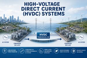
Transient stability analysis is one of the most critical assessments in modern power system engineering. It evaluates whether a power system can maintain synchronism following a large disturbance — such as a short-circuit fault, sudden load rejection, or generation trip — within the first few seconds after the event. For systems incorporating High Voltage Direct Current (HVDC) links, this analysis becomes significantly more nuanced because the DC transmission element responds to disturbances through fundamentally different physics than conventional AC machines.
Traditional transient stability analysis focuses entirely on synchronous machine rotor angle dynamics, governed by the classical swing equation. When an HVDC link is embedded within the AC network, the converter stations at each terminal introduce controllable active and reactive power exchange points that interact continuously with the surrounding AC buses. These interactions can either amplify or dampen electromechanical oscillations depending on how the converter controllers are configured.
The principal advantage of HVDC links from a stability perspective is their inherent controllability. Unlike AC transmission, where power flow is determined by network impedances and voltage angles, the power transferred through an HVDC link is governed by the firing angle of the thyristor valves (in line-commutated converters) or the modulation index of the switching devices (in voltage-source converters). This rapid and precise controllability makes HVDC a powerful tool for transient stability enhancement when appropriately integrated into the overall system control architecture.
Converter Model for Transient Stability Studies
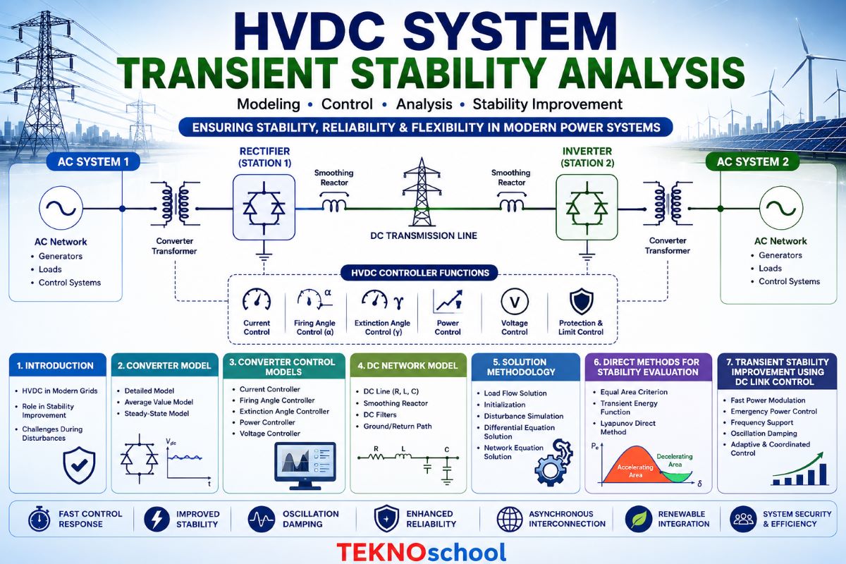
In transient stability simulations, HVDC converters are represented using quasi-steady-state (QSS) models rather than detailed electromagnetic transient (EMT) models. This simplification is justified because electromechanical dynamics in the AC network evolve over timescales of hundreds of milliseconds to several seconds, whereas the switching transients inside the converter valves resolve in microseconds. Representing every switching event would make system-wide stability simulation computationally prohibitive.
For a 12-pulse LCC converter, the quasi-steady-state DC voltage at the rectifier terminal is expressed as:
Where Vd0 is the ideal no-load DC voltage proportional to the AC bus voltage, α is the firing advance angle, Xc is the commutation reactance, and Idc is the direct current. The commutation reactance accounts for the overlap angle effect, representing the voltage reduction caused by finite commutation inductance. Reactive power consumed by an LCC converter is approximated as Q = P · tan(φ), where the power factor angle φ depends on both α and the commutation overlap angle μ.
At the inverter, the same formulation applies using the extinction advance angle γ instead of α. The constraint γ ≥ γmin (typically 15° to 18°) must be enforced throughout the simulation to prevent commutation failure — a condition where a valve fails to commutate current and the converter temporarily collapses.
A VSC converter is modelled as a controlled voltage source behind a phase reactor. The converter terminal voltage Vc is expressed in d-q components referenced to the AC bus voltage vector. The active and reactive power injections into the AC network are:
Q = (Vac / XL) · (Vac − Vc · cos(δ))
Here XL is the phase reactor impedance and δ is the angle between converter and AC bus voltages. VSC models are bounded by the converter current limit Imax and the DC voltage rating, both of which must be enforced as inequality constraints within each simulation timestep.
Converter Controller Models
Controller dynamics are explicitly represented in transient stability simulations because their time constants fall within the electromechanical timescale. A hierarchical structure governs both LCC and VSC converters.
| Control Level | Function | Typical Time Constant |
|---|---|---|
| Firing Pulse / Modulation | Direct gate pulse generation; fastest inner loop | <1 ms (not modelled in TSA) |
| Current / Power Control | PI regulators tracking Idc or Pdc reference | 10 – 100 ms |
| Voltage / Reactive Power | AC bus voltage regulation or Q dispatch | 50 – 300 ms |
| Power Order / Modulation | System-level power scheduling and stability modulation signals | 100 ms – seconds |
For LCC-HVDC, the rectifier station normally operates under constant current control (CCC), maintaining a DC current set-point regardless of AC system fluctuations. The inverter operates under constant extinction angle (CEA) control or constant voltage control. A voltage-dependent current order limiter (VDCOL) reduces the current reference when AC bus voltage falls below a threshold — typically 0.85 to 0.90 pu — preventing commutation failures during AC faults and accelerating recovery.
The voltage-dependent current order limiter is critical during fault recovery. Without VDCOL, the constant current controller demands full rated current into a depressed AC voltage, which prolongs the fault and risks consecutive commutation failures. The VDCOL characteristic is modelled as a piecewise linear function: the current order remains at the rated value above Vac = 0.9 pu, reduces linearly to a minimum (typically 0.3–0.4 pu rated) at Vac = 0.4 pu, and is clamped at the minimum below that voltage. This characteristic must be accurately represented in the controller model to correctly predict post-fault recovery behaviour.
For VSC-HVDC, inner current controllers operate in the d-q synchronous reference frame, producing fast and decoupled regulation of active and reactive currents. Outer controllers set the d-axis current reference to regulate active power or DC voltage, and the q-axis current reference to regulate AC bus voltage or reactive power. Phase-locked loop (PLL) dynamics are sometimes included for weak-grid studies where the converter terminal voltage angle may deviate significantly during a disturbance.
DC Network Model
The DC network connects the two (or more) converter stations through transmission cables or overhead lines, together with smoothing reactors and DC capacitors. For point-to-point HVDC, the DC network is often simplified to a lumped-parameter representation — a series resistance and inductance with lumped capacitance to ground at each terminal bus.
The dynamic behaviour of DC current in the smoothing reactor is described by:
Where Vdr and Vdi are the rectifier and inverter DC voltages, Rdc is the total DC line resistance, and Ldc includes both the line inductance and the smoothing reactor inductance. This first-order ODE is integrated simultaneously with the AC network power flow equations and the synchronous machine swing equations.
For multi-terminal DC (MTDC) networks with multiple nodes, the DC network is represented by a full nodal admittance matrix Ydc, analogous to the Y-bus matrix used for the AC network. Each DC bus has a capacitance to ground that stores energy and buffers voltage fluctuations. The nodal equations are:
Where Iconv is the vector of converter current injections, Cdc is the diagonal capacitance matrix, and Vdc is the DC nodal voltage vector. The DC capacitance provides an energy buffer that allows DC voltage to change gradually, maintaining converter controllability even when AC-side conditions fluctuate rapidly. Overhead DC lines may additionally be modelled as distributed-parameter π-sections when DC line fault studies are also intended.
Solution Methodology
The overall system for transient stability simulation consists of coupled differential-algebraic equations (DAEs). The differential equations describe the dynamics of synchronous machines, excitation systems, governors, and DC network elements. The algebraic equations represent the instantaneous power balance at every AC bus — the network power flow equations — which must be satisfied at every simulation timestep.
For a combined AC/DC system, the solution proceeds in a partitioned sequential approach at each timestep:
The partitioned sequential approach can suffer from interface errors between the AC and DC sub-solvers, particularly during rapid transients when both sub-systems change significantly within one timestep. Simultaneous solution methods — treating all AC and DC equations as a single unified nonlinear algebraic system — improve accuracy but increase computational cost due to the expanded Jacobian matrix. Predictor-corrector schemes provide a practical middle ground, using a predicted solution to initialize the Newton iteration and achieving convergence in fewer iterations.
Direct Methods for Stability Evaluation
Time-domain simulation reveals whether a particular fault scenario leads to stability or instability, but it does not directly quantify the stability margin. Direct methods, rooted in Lyapunov stability theory, address this limitation by computing an energy-based measure of how close the post-fault trajectory comes to the boundary of the stability region.
The transient energy function (TEF) method constructs a Lyapunov function V(δ, ω) that is positive definite in the region of interest and decreases along system trajectories during the post-fault period. For a simple two-machine equivalent, the TEF takes the form:
Where the first term is the kinetic energy of the rotor, the second and third terms are potential energy components relative to the stable equilibrium point δs. The critical energy Vcr is evaluated at the relevant unstable equilibrium point (UEP) — the closest point on the stability boundary in the direction of the fault trajectory. The transient energy margin is then:
A positive ΔV indicates the system is stable; a negative value indicates instability. The magnitude of ΔV provides a quantitative stability margin that can be used to rank contingencies and determine critical clearing times without performing multiple time-domain simulations.
The primary limitation of the TEF method is the difficulty in identifying the correct controlling UEP for multi-machine systems. The number of UEPs grows exponentially with the number of machines, and selecting the wrong UEP leads to overly optimistic or pessimistic stability assessments. Extended equal-area criterion (EEAC) methods and the boundary of stability region-based controlling UEP (BCU) method address this by systematically identifying the relevant UEP along the fault-on trajectory projected onto the reduced-state space.
Incorporating the HVDC link into the TEF framework requires augmenting the energy function to account for the energy stored in the DC network (primarily in smoothing reactor inductance and DC capacitors) and the dissipation in DC resistance. The converter power injections — which change with controller action — appear as path-dependent terms in the energy function, complicating the construction of a closed-form Lyapunov function. Current research addresses this by treating the DC power injection as a controllable parameter within the TEF framework, effectively updating the stable equilibrium point at each timestep to account for the changed operating condition imposed by the DC control.
Transient Stability Improvement Using DC Link Control
The rapid controllability of HVDC power transfer provides a unique opportunity to actively improve transient stability — an advantage unavailable to fixed-impedance AC transmission paths. When an AC system fault causes generator rotor angles to accelerate, the HVDC link can be modulated to reduce accelerating power in the faulted area and increase it at the receiving end, effectively applying a braking torque to the accelerating machines without requiring any physical braking resistor.
When a severe AC fault is detected, the DC power order is stepped up to maximum rated value to absorb excess mechanical energy from accelerating generators. The power increase is initiated within one to two cycles of fault detection, exploiting the HVDC link’s ability to bypass the stability limitation of the parallel AC corridor. EPC is implemented as a discrete control action triggered by fault detection signals, AC voltage magnitude deviation, or frequency deviation exceeding a preset threshold.
A supplementary modulation signal derived from system frequency deviation Δf or its derivative df/dt is superimposed on the DC power order reference. This signal acts analogously to a power system stabilizer (PSS) for the HVDC link, providing continuous damping of inter-area oscillations. The gain and phase characteristics of the modulation controller are designed to produce a damping torque component in phase with rotor speed deviation, using the same eigenvalue-based techniques applied to PSS design.
VSC-HVDC converters can supply reactive current independently of active power, making them capable of supporting AC bus voltage during and immediately after a fault. By rapidly injecting reactive current in proportion to voltage depression, the VSC converter effectively acts as a STATCOM, accelerating voltage recovery and reducing the risk of delayed fault clearance or cascading voltage collapse. Priority can be given to reactive current during the fault period and then seamlessly transferred back to active power modulation post-fault.
Coordinated runback schemes rapidly reduce DC power when a generation unit trips in the sending-end AC system, preventing the AC area from becoming excessively overloaded. Conversely, runup schemes increase DC power when a major load is suddenly disconnected, supplying load quickly via the DC link to prevent frequency overshoot. These schemes use SCADA or wide-area measurement system (WAMS) signals to initiate coordinated actions across both converter stations simultaneously.
Effective stability improvement through DC link control requires careful coordination between the HVDC control system and the AC system protection relays. Emergency power control actions must be fast enough to prevent loss of synchronism (response within 50–100 ms of fault onset) but must also include rate-of-change limiters to avoid exciting DC line resonances or inverter commutation failures. Wide-area measurement systems using phasor measurement unit (PMU) data at key AC buses provide the highest-fidelity input signals for modulation controllers, enabling responses proportional to the global electromechanical swing rather than local bus measurements alone.
Summary of Key Modelling Elements
| Component | Model Type in TSA | Key Parameter | Stability Role |
|---|---|---|---|
| LCC Converter | QSS algebraic + VDCOL | α, γmin, Vd0 | Active power transfer; reactive demand |
| VSC Converter | Controlled voltage source + d-q limits | Imax, XL, PLL bandwidth | P and Q independent control; voltage support |
| DC Network | First-order ODE (lumped L, R, C) | Ldc, Rdc, Cdc | Current smoothing; energy buffer |
| Converter Controller | PI regulators + limiters | Kp, Ki, VDCOL breakpoints | Recovery speed; fault ride-through |
| Stability Modulation | Supplementary signal on P-order | Gain, phase lead, washout time | Electromechanical oscillation damping |