Components Model for Analysis of AC DC Systems
Components Model for Analysis
of AC DC Systems
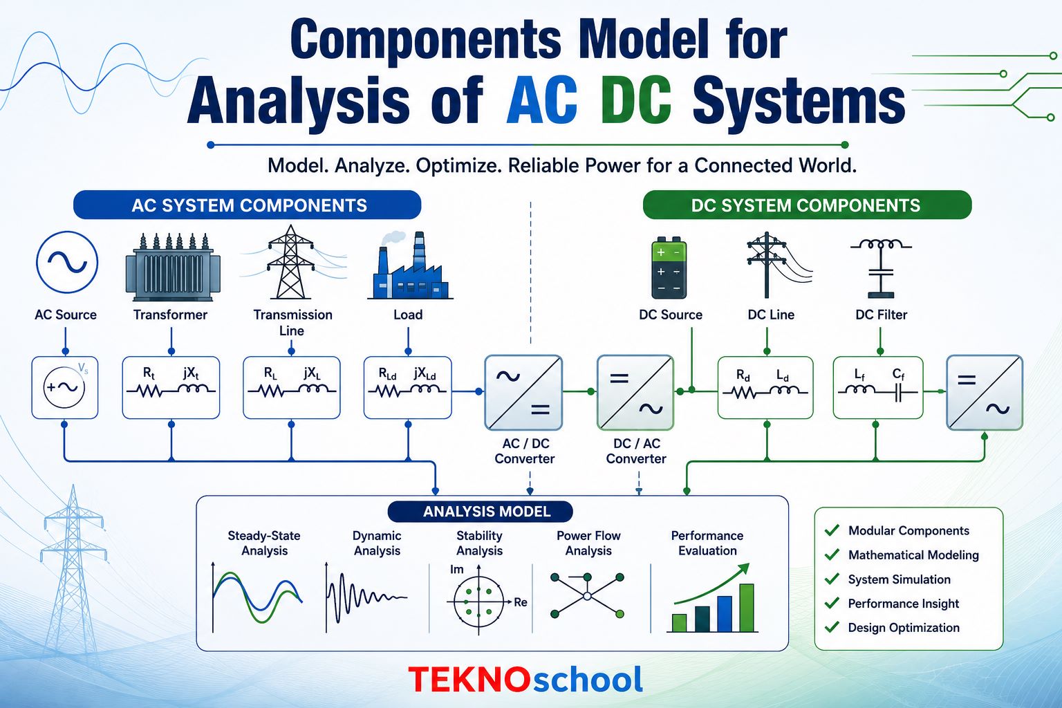
Components Model for Analysis of AC DC Systems- A structured framework covering converter modelling, control hierarchies, and the separate representation of AC and DC network elements for accurate steady-state and dynamic simulation.
The integration of High Voltage Direct Current (HVDC) transmission into modern power networks demands a rigorous modelling methodology that captures the behaviour of both the alternating-current and direct-current subsystems simultaneously. Classical AC power-flow tools are insufficient on their own because they cannot capture the nonlinear, discrete switching actions of the converters that couple the two domains.
The components model approach addresses this gap by decomposing the AC/DC system into distinct, interacting subsystems — the converter itself, its control system, the surrounding AC network, and the DC network — each described by equations appropriate to its physical nature. This modular decomposition simplifies both mathematical formulation and software implementation and allows each subsystem to be validated independently before being assembled into a unified simulation.
In steady-state power flow analysis, the components model is typically solved iteratively using an alternating or unified solution strategy. In dynamic simulation, each component contributes its own set of differential or algebraic equations, and the overall system is integrated forward in time. Understanding what each component model contains — and how the components exchange information at their interfaces — is the essential first step in any AC/DC system study.
Representing the AC/DC Interface
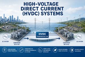
The converter — whether a line-commutated converter (LCC) or a voltage source converter (VSC) — is the element that translates between the AC and DC worlds. Its model must correctly reproduce the power exchange between the two domains, the reactive power demand imposed on the AC bus, and the harmonic currents injected into the AC network.
For a six-pulse or twelve-pulse LCC bridge, the fundamental-frequency steady-state model relates the DC voltage Vd to the AC bus voltage Vac, the transformer turns ratio, the commutation reactance Xc, and the firing angle α through the well-known relationship:
Vd = Vd0 cos α − (3/π) Xc Id
where Vd0 = (3√2/π) · (Vac / √3) · n is the ideal no-load DC voltage
The reactive power consumed by the converter is modelled as a function of the power factor angle φ, which is itself determined by the extinction angle γ (for inverter operation) or the firing angle α (for rectifier operation). This reactive power demand is a load imposed directly on the AC bus to which the converter transformer is connected, making its accurate representation critical for AC voltage stability studies.
For VSC-based HVDC systems, the converter model shifts from a phase-controlled to a pulse-width-modulated framework. The VSC is represented as a controllable voltage source behind a phase reactor. Its active power output and reactive power exchange are independently controllable through the modulation index and the phase angle of the converter voltage vector relative to the AC bus voltage. This decoupled control capability gives VSC converters a fundamentally different interaction with the AC network compared to LCC systems.
In both cases, the converter model provides the AC network with a current injection or an equivalent admittance, and provides the DC network with a voltage source or current source at the DC terminals. The consistency of power balance across this interface — ensuring that AC-side power equals DC-side power plus losses — must be enforced in every iteration of the solution.
Hierarchy of Control Functions
The control model governs what the converter does with its switching freedom — it determines the firing angle, the modulation index, or the valve-blocking logic at any given instant. In a components model framework, the control is separated from the converter power circuit so that alternative control strategies can be substituted without changing the fundamental converter equations.
| Control Level | Function | Typical Time Range |
|---|---|---|
| Valve Firing / Modulation | Generates gate pulses; determines α or PWM pattern | Microseconds to milliseconds |
| Inner Current Control | Tracks current reference; limits commutation failures | Milliseconds |
| Outer Power / Voltage Control | Regulates DC current, DC voltage, or AC voltage | Tens of milliseconds |
| System / Dispatch Control | Sets power order; coordinates multi-terminal HVDC | Seconds to minutes |
In steady-state power flow, only the outermost control level is relevant — the power order and the control mode specification (constant current, constant power, or constant voltage at the DC bus) determine the operating point. The inner control loops are assumed to have settled to their commanded values, so they are not explicitly represented.
In dynamic simulation, each layer of the control hierarchy is modelled with its own transfer functions and limiters. The interaction between the inner current controller and the outer power controller — particularly the current error amplifier (CEA) and the voltage-dependent current order limiter (VDCOL) in LCC systems — is critical for reproducing the system response to AC network disturbances and recovery behaviour following DC line faults.
Admittance Matrix and AC Bus Equations
The AC network model encompasses all transmission lines, shunt elements, transformers, and generators connected to the system. In the components model framework, the AC network is represented by its nodal admittance matrix Ybus, augmented to include the converter transformer impedances. Each converter terminal bus appears as a standard node within this matrix.
The power balance equations at every AC bus take the standard form of the active and reactive power mismatch equations used in Newton-Raphson load flow. At converter buses, an additional constraint must be incorporated — the relationship between the converter’s reactive power demand and the bus voltage — which couples the AC and DC solution spaces.
Transmission Network
Lines are represented by π-equivalent circuits with series impedance and shunt susceptance. Transformers include off-nominal tap ratios and phase-shift angles incorporated directly into the Ybus elements.
Reactive Compensation
Switched capacitor banks and filters at converter stations are modelled as shunt admittances at the converter bus. Their switching states must be updated as part of the outer control loop to satisfy reactive power targets.
Generator Models
In steady-state, generators are represented as PV or slack buses. In dynamic simulation, full machine models with excitation and governor systems are coupled to the AC network through voltage-current interface equations.
Short-Circuit Strength
The short-circuit ratio (SCR) at the converter bus, derived from the AC Thevenin impedance, determines the sensitivity of the AC voltage to converter current injections and governs commutation performance for LCC systems.
In dynamic analysis, the AC network model is often represented as an algebraic set of equations (assuming quasi-static phasors) because electromagnetic transients on transmission lines settle far faster than the electromechanical and control dynamics of primary interest. This phasor approximation substantially reduces computation time while preserving the accuracy needed for stability studies.
DC Line, Smoothing Reactor, and Filters
The DC network consists of the overhead DC line or cable, the smoothing reactor at each converter terminal, and any DC-side harmonic filters. Unlike the AC network, the DC network carries no reactive power, and its behaviour is governed by resistive-inductive dynamics rather than by phasor power flow equations.
For steady-state analysis, the DC network is modelled as a pure resistance network. The DC line resistance Rdc — which includes conductor resistance corrected for skin effect and temperature — and the smoothing reactor (treated as lossless in steady state) together form a simple voltage divider between the rectifier and inverter DC terminals. The power balance equation then takes the form:
Vdr − Vdi = Id · Rdc
where subscripts r and i denote rectifier and inverter terminals respectively
In dynamic simulation, the DC network is represented by its full differential equations. The smoothing reactor with inductance Ld and the DC line distributed parameters — modelled as a lumped π section or as a cascade of π sections for more accurate travelling-wave representation — yield a set of first-order differential equations governing the evolution of DC current and the voltage across the line capacitance. The smoothing reactor dynamics are particularly important during fault recovery, since the large inductance limits the rate of change of DC current and introduces a characteristic time constant that defines the speed of the control system response.
Smoothing Reactor
Limits current ripple and rate-of-rise during faults. Typically, several hundred millihenrys. Its inductance appears in the DC current differential equation as dId/dt = (Vdr − Vdi − IdRdc) / Ld.
DC Line / Cable
For overhead lines, lumped-π representation is adequate for frequencies below a few hundred hertz. Underground cables require frequency-dependent models due to the much larger capacitance and the significance of skin-effect losses.
DC Filters
Tuned LC circuits are placed on the DC side to suppress characteristic harmonics (12th, 24th, etc.) from being impressed onto the DC line. In stability studies, these are often omitted; in harmonic studies, they must be explicitly represented.
For multi-terminal DC (MTDC) systems, the DC network model expands to include multiple converter terminals connected by a meshed DC grid. A DC admittance matrix analogous to the AC Ybus can be formulated, and the DC nodal voltage equations are solved simultaneously with the converter and control equations. Power flow control in MTDC networks requires additional constraints — such as droop characteristics on the DC voltage-power relationship at each converter — to be incorporated into the model.
The components model framework achieves its greatest value when these four subsystems — converter, control, AC network, and DC network — are consistently coupled through clearly defined interface variables. The rectifier bus AC voltage and the DC terminal current are the primary exchange quantities at every converter interface, and maintaining their consistency across subsystems is the central task of any AC/DC load flow or dynamic simulation algorithm.