Digital Dynamic Simulation of HVDC Systems
Digital Dynamic Simulation of HVDC Systems
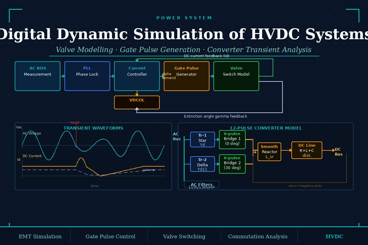
Dynamic Simulation-A complete engineering framework — from simulation philosophy and valve modelling through gate pulse generation, converter representation, and full transient analysis of AC/DC networks.
Simulation Philosophy and Digital Tool Framework
The digital simulation of HVDC systems is governed by a fundamental engineering philosophy: every component of the converter station — the thyristor valve, the converter transformer, the smoothing reactor, the AC filters, the DC line — must be represented with sufficient fidelity to capture the phenomenon under study, without introducing unnecessary computational burden. This balance between accuracy and efficiency shapes every decision in the simulation framework.
HVDC simulation tools fall into two broad categories based on their mathematical foundations. Electromagnetic Transient (EMT) programs — of which PSCAD/EMTDC, EMTP-RV, and ATP-EMTP are the most widely used — solve the network differential equations at every time step using numerical integration methods such as the trapezoidal rule. These tools resolve the sub-millisecond switching transients, commutation notches, and harmonic content that define converter behaviour with high fidelity. Transient stability programs, by contrast, represent converters through algebraic average-value models and are suited to studying electromechanical phenomena over timescales of seconds.
The selection of a simulation tool is therefore study-dependent. Commutation failure analysis, valve stress studies, harmonic filter design, and protection system testing demand EMT-level detail. Power flow control, stability margin assessment, and inter-area oscillation damping studies can be adequately addressed with average-value models. Many modern HVDC simulation workflows employ both — an EMT model for detailed converter validation and a reduced average-value model embedded within a large transient stability network for system-level studies.
The simulation time step is the single most important parameter in EMT-based HVDC simulation. A time step of 20 to 50 microseconds is typically required to accurately resolve commutation transients in a 50 Hz system. Larger time steps miss the extinction angle dynamics and produce incorrect commutation failure predictions; smaller steps increase computation time without meaningful accuracy gain. The choice of 50 microseconds corresponds to approximately 1/400th of the fundamental period — providing adequate resolution of harmonic content up to the 200th order.
Valve Model
The thyristor valve is the fundamental switching element of an LCC-HVDC converter. In a 12-pulse converter station, twelve valves are arranged in two six-pulse bridges connected in series on the DC side and supplied by two converter transformers with different secondary winding connections — one star and one delta — to achieve 30-degree phase displacement between the two bridges. Each valve in a high-voltage HVDC station comprises a series string of hundreds of thyristors, but for simulation purposes, the entire valve is represented as a single controlled switching element.
The valve model in an EMT simulation captures three distinct operating states: the forward-blocking state, in which the valve holds off positive anode-to-cathode voltage without conducting; the conducting state, in which the valve carries DC current with a small forward voltage drop; and the reverse-blocking state, in which the valve extinguishes after current falls to zero and then holds off negative voltage. The transition from blocking to conducting is triggered by the gate pulse; the transition from conducting to reverse-blocking occurs naturally when the commutating AC voltage reverses the current through the valve, and it reaches zero.
Forward-blocking state: The valve is modelled as a very high resistance — typically 10 megaohms — in parallel with a small snubber RC circuit. The snubber (typically 0.01 microfarad in series with 20 ohms per thyristor level) limits the rate of rise of voltage during forward recovery and damps oscillations following a missed firing pulse.
Conducting state: The valve is modelled as a low resistance — typically 0.01 ohms — representing the aggregate on-state resistance of all thyristors in the series string, plus a voltage source representing the net forward voltage drop. This drop is typically 1 to 2 volts per thyristor level, and in a valve of 80 to 150 thyristors in series it contributes a measurable but modest power loss term.
Reverse-blocking state: After current extinction, the valve switches back to the high-resistance blocking model. The extinction angle gamma is calculated at every time step as the electrical angle elapsed since the last current zero crossing of the valve. This computed gamma is the primary input to the inverter constant extinction angle controller and to commutation failure detection logic.
For VSC-HVDC simulation, the valve model is substantially different. IGBT-based valves are modelled as bidirectional switches with anti-parallel diodes. In detailed models, each IGBT is represented individually with switching loss characteristics. In average-value models, the entire converter leg is replaced by a controlled voltage source whose magnitude and phase are determined by the modulation index and phase angle commands from the upper-level controller. This abstraction eliminates individual switching events and allows much larger simulation time steps — typically 100 to 500 microseconds — while still capturing the fundamental frequency and low-order harmonic behaviour.
The snubber circuit parameters must be chosen carefully. An overly large snubber capacitance slows the valve voltage rise after firing and produces unrealistically smooth commutation notches; an overly small capacitance allows high-frequency numerical oscillations to develop at valve turn-off. These oscillations are purely a simulation artefact and do not represent physical behaviour, but they can trigger spurious gate pulses if the firing control logic monitors valve voltage directly.
Gate Pulse Generation
Gate pulse generation is the mechanism by which the HVDC control system translates a firing angle demand — expressed as an electrical angle alpha relative to the natural commutation voltage zero crossing — into a physical gate trigger signal delivered to the appropriate thyristor valve at the correct instant. The accuracy and robustness of gate pulse generation directly determines converter performance under both steady-state and disturbed conditions.
The natural commutation voltage zero crossing for each valve is derived from the AC bus voltage at the converter transformer primary or secondary terminals. In simulation, a Phase-Locked Loop (PLL) tracks the AC voltage fundamental frequency and phase angle continuously, providing a synchronised angular reference against which the firing angle alpha is measured. The PLL output is a ramp signal that increases linearly from zero to 360 degrees over each fundamental cycle, resetting at each positive zero crossing of the reference phase.
Equidistant pulse firing (EPF): All six valves in a six-pulse bridge receive gate pulses spaced exactly 60 degrees apart in time, regardless of the actual AC voltage waveform. The firing interval is derived from a voltage-controlled oscillator locked to the AC system frequency. EPF produces uniform harmonic spectra and is less sensitive to AC voltage unbalance, but cannot compensate for asymmetric AC supply conditions.
Individual phase control (IPC): Each valve’s firing instant is determined independently from the zero crossing of its own commutating voltage, with alpha measured from that zero crossing. IPC responds correctly to asymmetric AC conditions and voltage distortions, but produces non-equidistant pulses under unbalanced supply, generating non-characteristic harmonics — particularly 2nd, 4th, and 6th order — that must be accounted for in filter design.
In the simulation model, gate pulses are generated by comparing the PLL output ramp angle against the demanded firing angle alpha at every time step. When the ramp angle equals alpha for the valve due to fire next in the firing sequence, a gate pulse is issued. The pulse is maintained for a minimum hold-on time — typically 120 electrical degrees — to ensure the valve remains triggered even if the current attempts to extinguish prematurely due to commutation difficulties. Simultaneously, the valve firing sequence controller advances its pointer to the next valve in the firing order, ready for the next firing event.
Alpha minimum and alpha maximum limiters are implemented within the gate pulse generation block. For the rectifier, alpha_min is typically 5 degrees to prevent firing too close to the natural commutation voltage zero and to protect against voltage spikes. For the inverter, the firing angle is controlled indirectly through the gamma controller, with the effective firing angle bounded between approximately 100 and 165 degrees. These limits are enforced in the simulation at the gate pulse generation stage, not in the outer control loops.
Generation of Control Voltage
The control voltage — also referred to as the firing control signal or the alpha demand voltage — is the output of the HVDC master controller that specifies the firing angle required to achieve the desired DC current or DC voltage operating condition. Understanding how this control voltage is generated within the simulation is essential to correctly representing HVDC dynamic behaviour during both normal operation and transient events.
At the rectifier, the control voltage is generated by a current controller that compares the measured DC current (Id_measured) against the DC current reference (Id_ref) and outputs a firing angle adjustment through a proportional-integral (PI) regulator. The PI output is the alpha demand signal. An increase in alpha reduces the rectifier DC voltage, reducing the current; a decrease in alpha raises the DC voltage and current. The PI gains and integrator time constants must be tuned to match the electrical time constants of the DC circuit — primarily determined by the smoothing reactor inductance and the DC line resistance.
Step 1 — Current error computation: Id_error = Id_ref minus Id_measured. The measured current is filtered through a low-pass filter with a time constant of 1 to 5 milliseconds to remove high-frequency switching ripple before the error is fed to the PI controller.
Step 2 — PI regulation: The PI controller integrates the current error and produces an alpha demand in degrees. Anti-windup logic prevents integrator saturation when the alpha demand hits its minimum or maximum limits — a critical implementation detail that is frequently absent in simplified simulation models, leading to incorrect recovery behaviour after fault clearance.
Step 3 — VDCOL modification: The Voltage Dependent Current Order Limiter modifies Id_ref downward when the DC voltage at the rectifier bus falls below a threshold — typically 0.4 per unit. The modified current order reduces the alpha demand proportionally, preventing the rectifier from attempting to maintain full current into a depressed DC voltage, which would drive alpha to its minimum and destabilise the DC circuit.
Step 4 — Alpha demand output: The final alpha demand is passed to the gate pulse generation block. Simultaneously, the alpha demand is monitored by protection logic that detects abnormal firing angles — for example, alpha exceeding 90 degrees at the rectifier during a severe AC fault — and initiates protective actions such as inverter bypass or DC line de-energisation.
At the inverter, the control voltage is generated by the gamma controller rather than a current controller. The gamma controller measures the actual extinction angle of the most recently extinguished valve and compares it against the gamma reference — typically 15 to 18 degrees. A PI regulator acting on the gamma error adjusts the inverter firing angle to maintain the desired gamma margin. The inverter current controller operates in parallel, reducing the inverter current order by a current margin — typically 0.1 per unit — below the rectifier current order, ensuring that under normal conditions the rectifier current controller is the active regulating loop.
Converter Transformer Model
The converter transformer is one of the most complex components to model accurately in an HVDC simulation. It serves three simultaneous functions: it provides galvanic isolation between the AC system and the converter; it steps down the AC system voltage to the converter valve voltage level; and through its leakage reactance, it controls the rate of current rise during commutation, determining the commutation overlap angle mu and therefore the DC voltage reduction under load.
In the standard simulation model, the converter transformer is represented by a two-winding ideal transformer with a series leakage impedance branch. The leakage reactance — expressed in per unit on the transformer MVA base, typically 0.12 to 0.20 per unit — is the dominant parameter. It appears directly in the commutation equation: the commutation overlap angle mu is determined by the DC current Id and the commutation reactance Xc, which equals the transformer leakage reactance referred to the converter side. A larger leakage reactance produces a larger overlap angle, greater DC voltage reduction under load, and a larger effective firing angle advance requirement at the inverter.
Basic linear model: Ideal transformer plus series RL leakage impedance. Adequate for steady-state commutation studies and most transient simulations. The magnetising branch is neglected; core saturation and inrush are not represented.
Saturable core model: The magnetising branch is represented by a nonlinear inductance whose flux-current characteristic follows the transformer’s measured saturation curve. This model is essential for energisation studies, where inrush currents of 6 to 10 times the rated current can saturate the core and generate large low-order harmonics that stress AC filters and may falsely operate differential protection relays.
Frequency-dependent model: At high frequencies, the transformer exhibits complex distributed capacitance effects between windings and from winding to ground. A frequency-dependent model using ladder network circuits represents these effects and is required for studies of fast-front transients, such as lightning surge propagation or disconnector switching in the converter hall.
The on-load tap changer (OLTC) of the converter transformer is modelled as a discrete step change in turns ratio, with a minimum step time of 5 to 10 seconds reflecting the mechanical operating time of the tap changer drive. In simulation, the OLTC controller monitors the firing angle alpha and adjusts the tap position to keep alpha within an optimal range — typically 12 to 17 degrees at the rectifier — so that the current controller has adequate modulation range. The tap changer interaction with the current controller is a slow outer loop that must be co-simulated with the converter control to correctly represent steady-state operating point establishment following a major disturbance.
Converter Model
The converter model integrates the transformer model, the valve models, the DC side components — smoothing reactor and DC line — and the gate pulse generation logic into a coherent network that is solved simultaneously at every simulation time step. In EMT programs, the solution method is based on companion circuit representations of all energy storage elements, converting inductors and capacitors into Norton equivalent circuits that are updated at each time step using the trapezoidal integration rule.
The 12-pulse converter model is assembled from two six-pulse bridge submodels — one supplied by the star-connected transformer secondary and one by the delta-connected secondary — with their DC sides connected in series. The 30-degree phase shift between the two secondary voltages causes the 12-pulse characteristic harmonics — the 11th, 13th, 23rd, and 25th on the AC side, and the 12th and 24th on the DC side — while cancelling the 5th, 7th, 17th, and 19th order harmonics that would be present in a six-pulse configuration. This harmonic cancellation is automatically represented in the simulation through the correctly phased transformer secondary voltages; no additional harmonic correction is needed in the model formulation.
The DC smoothing reactor must be included in the converter model as a separate lumped inductance element, not absorbed into the transformer leakage reactance. The smoothing reactor — typically 0.3 to 0.6 Henrys in a high-voltage system — limits the rate of rise of DC fault current during a DC line fault and provides the energy storage that maintains DC current continuity during commutation. Omitting or undersizing it in the simulation produces unrealistically fast fault current rises and incorrect commutation failure predictions during AC voltage dips.
AC harmonic filters are connected to the converter AC bus in the simulation model as parallel RLC branches, each tuned to a specific harmonic order. The 11th- and 13th-order filters are mandatory for a 12-pulse converter; high-pass filters cover the broadband harmonic content above the 24th order. These filter branches participate in the network solution at every time step and affect the AC bus voltage waveform seen by the converter transformer, making them integral to commutation accuracy rather than post-processing additions.
For average-value converter models used in transient stability programs, the converter is represented by two controlled sources: a DC voltage source whose magnitude equals the ideal no-load DC voltage (Vd0) multiplied by cosine of alpha, minus the commutation voltage drop term (3 times Xc times Id divided by pi); and a reactive power sink on the AC side whose magnitude is determined by the power factor angle of the converter. These algebraic relationships update instantaneously at each simulation time step, providing a computationally efficient representation at the cost of switching-level detail.
Transient Simulation of DC and AC Systems
Transient simulation brings together all the component models — valve, transformer, converter, control — into a unified time-domain network solution that captures the system’s response to disturbances. The range of disturbances studied covers both DC-side events and AC-side events, and the interactions between them are often where the most critical HVDC behaviour emerges.
DC line fault: A pole-to-ground or pole-to-pole fault on the overhead DC line produces a rapid collapse of DC voltage at the fault point and a travelling wave that reflects from the converter ends. The simulation must represent DC line distributed parameters — resistance, inductance, and capacitance per unit length — using either a frequency-dependent line model or a pi-section approximation. The rectifier responds by driving alpha to its maximum (typically 90 to 150 degrees) to force the DC voltage negative and extinguish the fault current, while the inverter may experience commutation failure due to the DC current overshoot that precedes extinction.
DC current step change: A step change in the DC current order — such as that commanded by a power modulation controller — produces a transient in the DC circuit determined by the smoothing reactor time constant (L_sr divided by R_dc). The simulation tracks the actual DC current as it follows the new order through the PI current controller and verifies that the firing angle trajectory remains within limits during the transition.
Converter blocking and deblocking: A blocked converter — all gate pulses inhibited — causes DC current to fall to zero as the smoothing reactor energy dissipates into the system resistance. The simulation verifies that the DC current reaches zero within the expected time frame and that the AC system voltage recovers without excessive transient overvoltage from the sudden removal of the reactive power load.
AC bus fault at the inverter: A three-phase or single-phase fault on the inverter AC bus depresses the commutating voltage, reducing the extinction angle of all conducting valves simultaneously. The simulation tracks gamma in real time; when gamma falls below the minimum safe value — typically 7 to 10 degrees — commutation failure is declared. During a commutation failure, two valves in the same bridge conduct simultaneously, short-circuiting the DC line and causing a rapid rise in DC current. The simulation must correctly model the sequential events: gamma reduction, commutation failure, DC current overshoot, rectifier alpha drive-up, fault current extinction, and system restart.
AC voltage unbalance: Unbalanced AC conditions — arising from single-phase faults or unequal loading — produce negative-sequence voltage components at the converter bus. These components create 2nd- and 4th-harmonic currents in the DC circuit and cause non-equidistant firing in individual-phase-controlled converters. The simulation captures this behaviour through the full three-phase transformer and valve model and is used to verify that the negative-sequence harmonic content remains within equipment ratings.
Generator trip and frequency deviation: Loss of a major generating unit at the rectifier end causes AC frequency to fall. The simulation captures the effect of frequency deviation on the PLL tracking performance, the resulting shift in firing angle timing, and the interaction between the HVDC current controller response and the AC frequency recovery. This study is particularly important for HVDC links connecting a weak generation system — such as a remote hydroelectric plant — to a large mainland grid.
Every HVDC digital simulation model must be validated against field measurements or physical simulator results before it is used for engineering decisions. The standard validation protocol compares the simulated DC voltage, DC current, AC bus voltage magnitude, firing angle alpha, and extinction angle gamma waveforms against corresponding commissioning test recordings — typically steady-state power ramp tests, step response tests, and fault recovery tests recorded during station commissioning. Discrepancies exceeding 5 percent in peak values or 10 electrical degrees in timing indicate model parameter errors that must be resolved before the simulation is used for protection setting calculation or system impact studies.
Key Takeaways
EMT tools resolve sub-millisecond switching transients at 20 to 50 microsecond time steps; average-value models serve stability studies. Tool selection must match the study objective.
Three-state valve switching with snubber circuits, PLL-synchronised gate pulses with alpha limits, and anti-windup PI control together define converter dynamic accuracy.
Leakage reactance governs commutation overlap; saturable core models are required for energisation studies; the smoothing reactor must never be omitted from the DC circuit model.
DC line faults, AC bus faults, commutation failure sequences, and frequency deviation studies each stress different model components. Field measurement validation against commissioning data is mandatory before engineering use.